
MACHINE LEARNING
Prof. Edier Aristizábal

Curso
Classroom
Class code: wv4cglx
Para tener acceso debera recibir una invitación del profesor. En caso de no recibirla por favor solicitar dicho acceso con un correo electrónico donde se identifique claramente el curso al cual hace referencia.

Página web
https://edieraristizabal.github.io/MachineLearning/ (...es esta misma página)Curso Machine Learning
El curso de Machine Learning está orientado para estudiantes de ingeniería que deseen adquirir conocimientos sobre modelos multivariados, para análisis de inferencia estadística y predicción de una variable dependiente a partir de variables independentes o predictoras.
Para dichos análisis se utilizarán técnicas de aprendizaje automático como:
- Machine Learning
- Data Mining
- Big Data
Las herramientas de procesamiento serán:
- Lenguaje de programación Python y R en Notebooks (*.ipnyb) a traves de Google Colab y/o Jupyter Lab distribuido por Conda
Curso Machine Learning
El curso de Machine Learning está enfocado en la construcción de modelos basados en datos espaciales, que ayuden a entender la distribución y comportamientos de procesos físicos en ciencias de la tierra.
No es un curso de Python, R o SIG, por lo tanto no requiere conocimientos profundos en dichas herramientas. El curso, sin entrar en detalle en los aspectos básicos de estas herramientas, parte que el estudiante conoce lo basico de dichas herramientas, no se requiere ser un experto. El curso es una construcción conjunta de conocimiento por parte tanto de los estudiantes como del profesor.
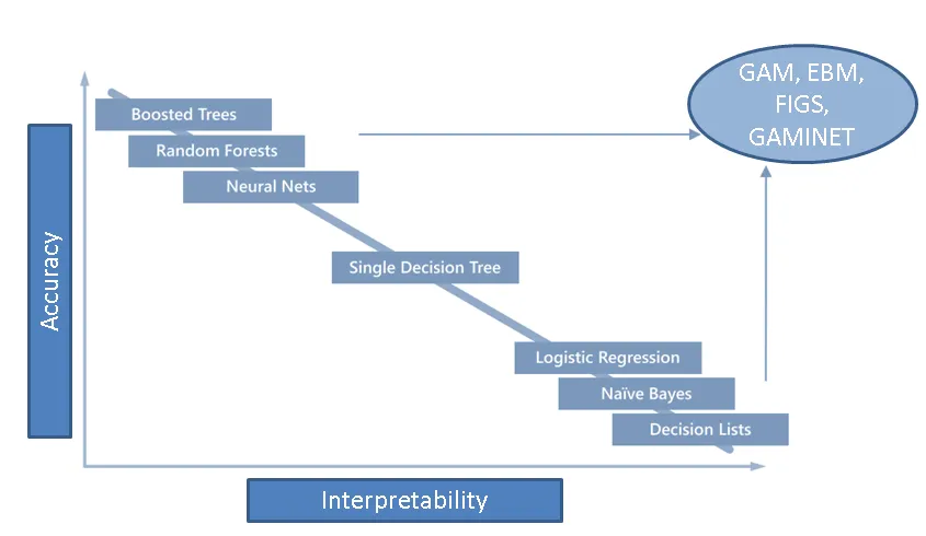
El enfoque del curso es el uso de análisis de datos espaciales y/o temporales para solucionar problemas en el campo de las geociencias, dando prioridad a modelos de datos que puedan interpretarse, y permitan brindar conocimiento del fenómeno físico
Cronograma y contenido del curso

Cronograma y contenido del curso

Evaluación del curso

“In God we trust. All others must bring data"
W. Edwards Deming (1900–1993)
Intro
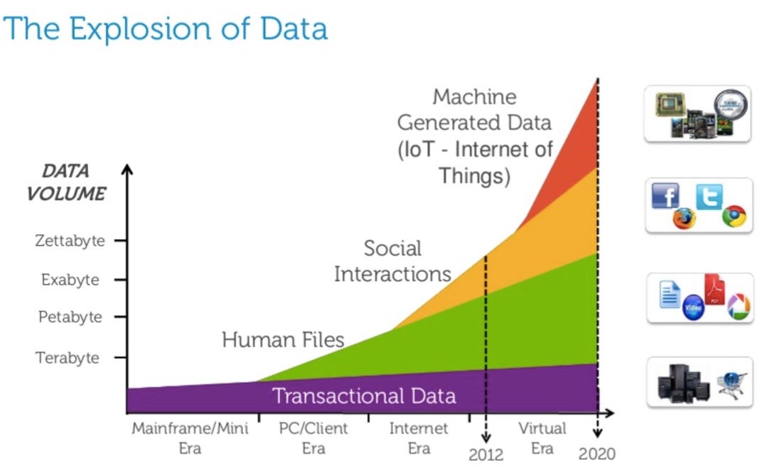
La era de los datos

Data store
Los kilobytes eran almacenados en discos, megabytes fueron almacenados en discos duros, terabytes fueron almacenados en arreglos de discos, y petabytes son almacenados en la nube.
(Anderson, 2008)


Inteligencia Artificial
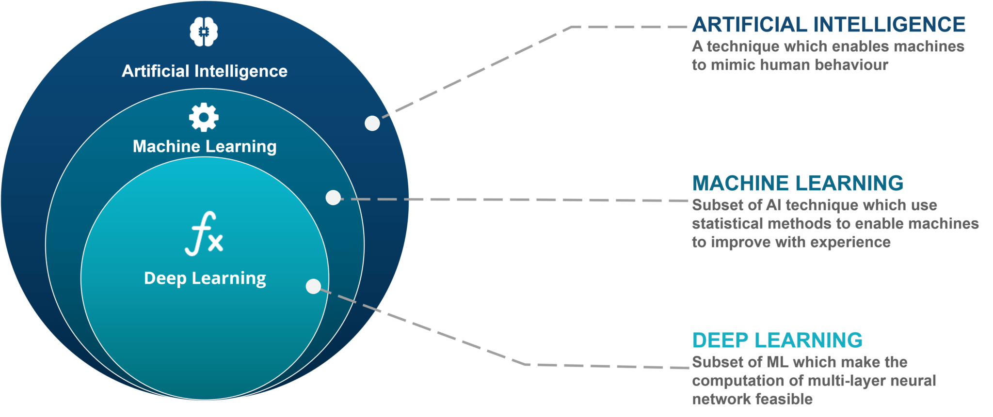
Inteligencia Artificial

Data science
Metodología y técnica para extraer información de datos en un dominio del conocimiento.

Data mining
The field of data mining involves processes, methodologies, tools and techniques to discover and extract patterns, knowledge, insights and valuable information from non-trivial datasets.
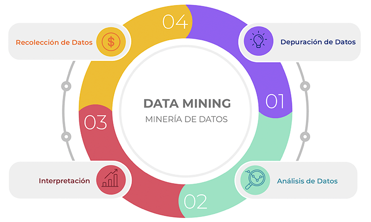
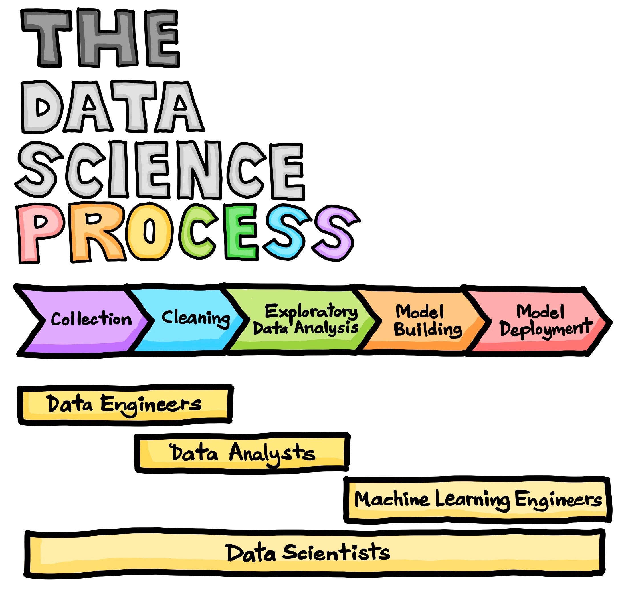
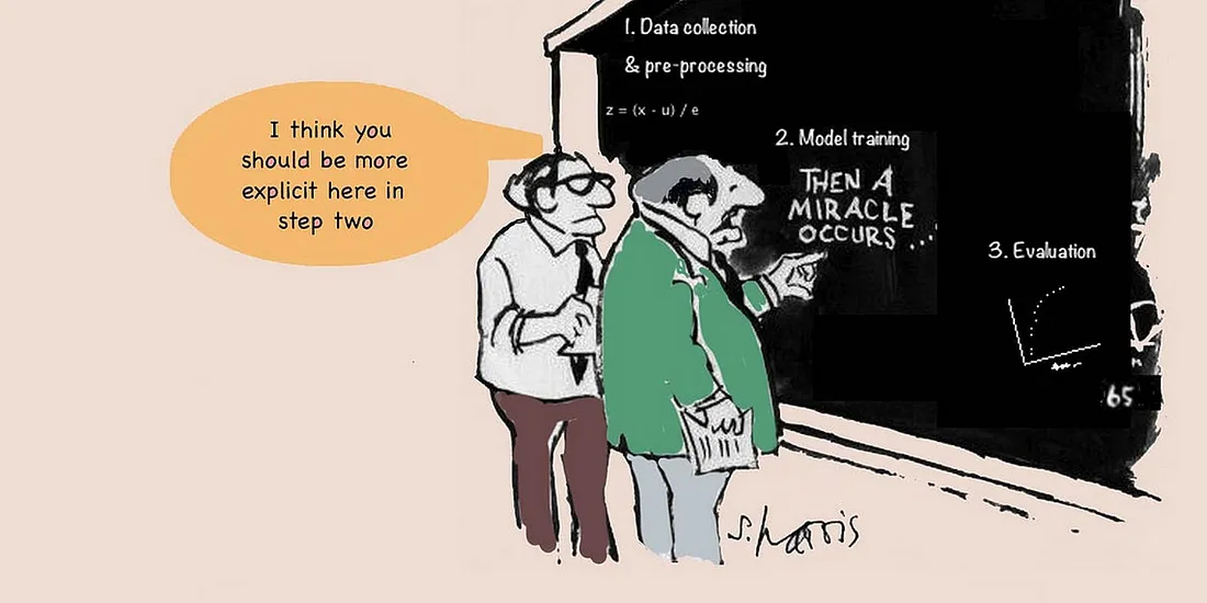
Data Science Lifecycle

Data Science Lifecycle

Machine learning
“A computer program is said to learn from experience E with respect to some class of tasks T and performance measure P, if its performance at tasks in T, as measured by P, improves with experience E.”

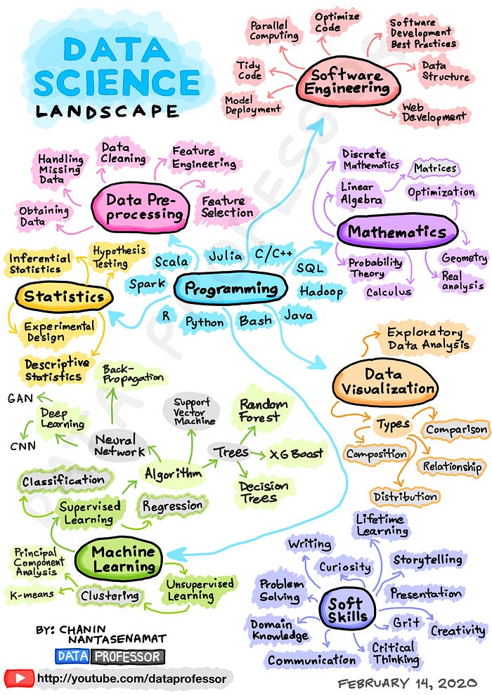
Machine learning...in this course

Data Science Lifecycle

Procesamiento general


Ambiente de trabajo
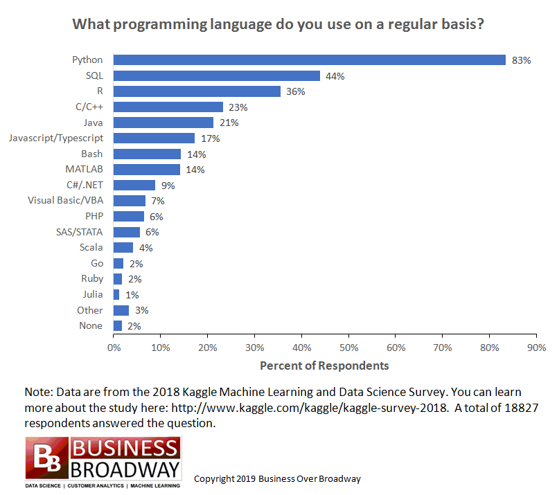
Programming lenguages for data science
R Lenguaje

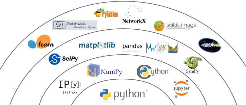
Python
Python code is fast to develop: As the code is not required to be compiled and built, Python code can be much readily changed and executed. This makes for a fast development cycle.
Python code is not as fast in execution: Since the code is not directly compiled and executed and an additional layer of the Python virtual machine is responsible for execution, Python code runs a little slow as compared to conventional languages like C, C++, etc.
It is interpreted: Python is an interpreted language, which means it does not need compilation to binary code before it can be run. You simply run the program directly from the source code.
It is object oriented: Python is an object-oriented programming language. An object--oriented program involves a collection of interacting objects, as opposed to the conventional list of tasks. Many modern programming languages support object-oriented programming. ArcGIS and QGIS is designed to work with object-oriented languages, and Python qualifies in this respect.
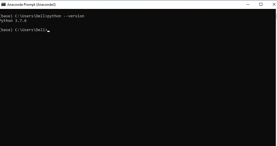
Python
Anaconda
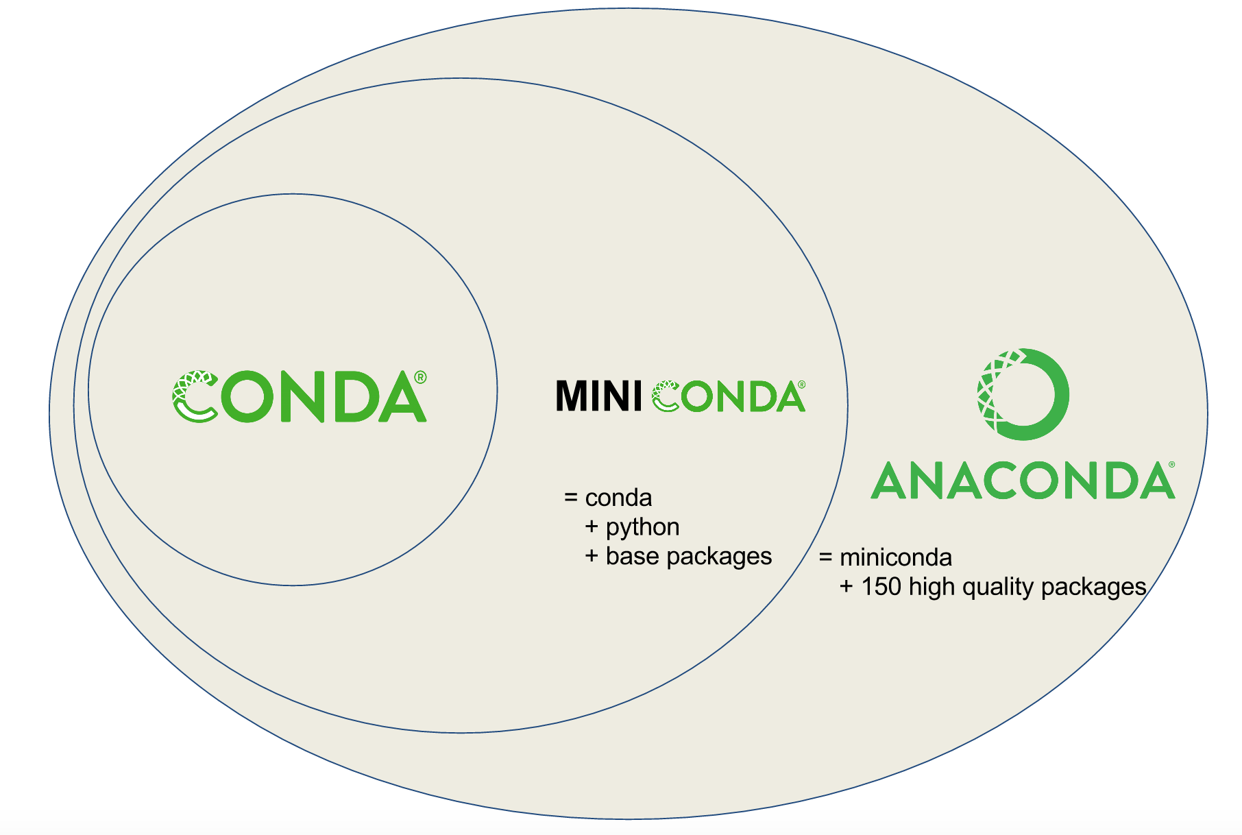
Anaconda


Miniconda
Python Packaging Index

Python Packaging Index

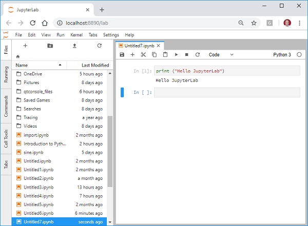
Jupyter Lab
Docker


Modelos basados en datos

Qué es un modelo?
A model is an an idealized representation of a system

Qué es un modelo?
Why do we build models?
- Models enable us to make accurate predictions
- Provide insight into complex phenomena

Qué es un modelo?


Black Box models
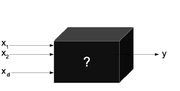
Modelos Explicativos
In this situation we wish to estimate $f$, but our goal is not necessarily to make predictions for $Y$. We instead want to understand the relationship between $X$ and $Y$ , or more specifically, to understand how $Y$ changes as a function of $X1, . . .,Xp.$
$\widehat{f}$ cannot be treated as a black box, because we need to know its exact form. In this setting, one may be interested in answering the following questions:
- Which predictors are associated with the response?
- What is the relationship between the response and each predictor?
- Can the relationship between $Y$ and each predictor be adequately summarized using a linear equation, or is the relationship more complicated?
Modelos Explicativos
Los modelos explicativos se refieren a la aplicación a datos de modelos estadísticos para verificar hipótesis causales sobre construcciones teóricas.
Los científicos están entrenados para reconocer que correlación es no causalidad, no es recomendable sacar conclusiones solo basado en la correlación entre $X$ y $Y$ (es posible que solo sea una coincidencia). Por lo tanto, se debe entender el mecanismo que subyace y que conecta $X$ y $Y$.
Modelos & Datos
En modelos explicativos, la función $\widehat{f}$ es cuidadosamente construida basada en $f$, en una forma que soporte interpretando la relación estimada entre $X$ y $Y$, y testeando la hipótesis causal.
- Datos reducidos: En los modelos basados en una cantidad de datos finitos, sí existe una diferencia significativa entre modelos explicativos y modelos predictivos, ya que un modelo óptimo para propósitos de predicción puede ser muy diferente a un modelo
- Big data: Puede no existir una diferencia significativa entre modelos explicativos y predictivos para inferir la verdadera estructura de la función $\widehat{f}$ o hacer predicciones cuando se cuenta con datos infinitos o si no existe ruido en los datos.
Asociación vs Correlación vs Causalidad
Association (dependence): indicates a general relationship between two variables, where one of them provides some information about another.
Correlation: refers to a specific kind of association and captures information about the increasing or decreasing trends (whether linear or non-linear) of associated variables.
Causation: refers to a stronger relationship between two associated variables, where the cause variable “is partly responsible for the effect, and the effect is partly dependent on the cause”.
- Statistical dependency does not imply causality
- Sometimes the existence of statistical dependencies between system inputs and outputs is (erroneously) used to demonstrate cause-and-effect relationship between variables of interest.
- Causality cannot be inferred from data analysis alone; instead, it must be assumed or demonstrated by an argument outside the statistical analysis.
Correlación vs Causalidad

Correlación vs Causalidad

No-Free-Lunch (D. Wolpert & W. Macready (1997)

No-Free-Lunch

“Data is useful to illuminate the path, but keep following the path to find the full story..."
Quién dijo esto?
Data processing
Data structures in machine learning
There are two basic types of data and one hybrid:
Cross-Sectional data: sample of observations on individual units taken at a single point in time. Individual observations have no natural ordering adn statistically independent.
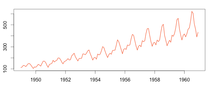
Time series data: consists of a sample of observations on one or more variables over successive periods of time. They have a chronological ordering.
Hybrid data structures: combine the inherent characteristics of cross-sectional and time-series data sets. They could be Pooled Cross-Section or Panel (longitudinal).
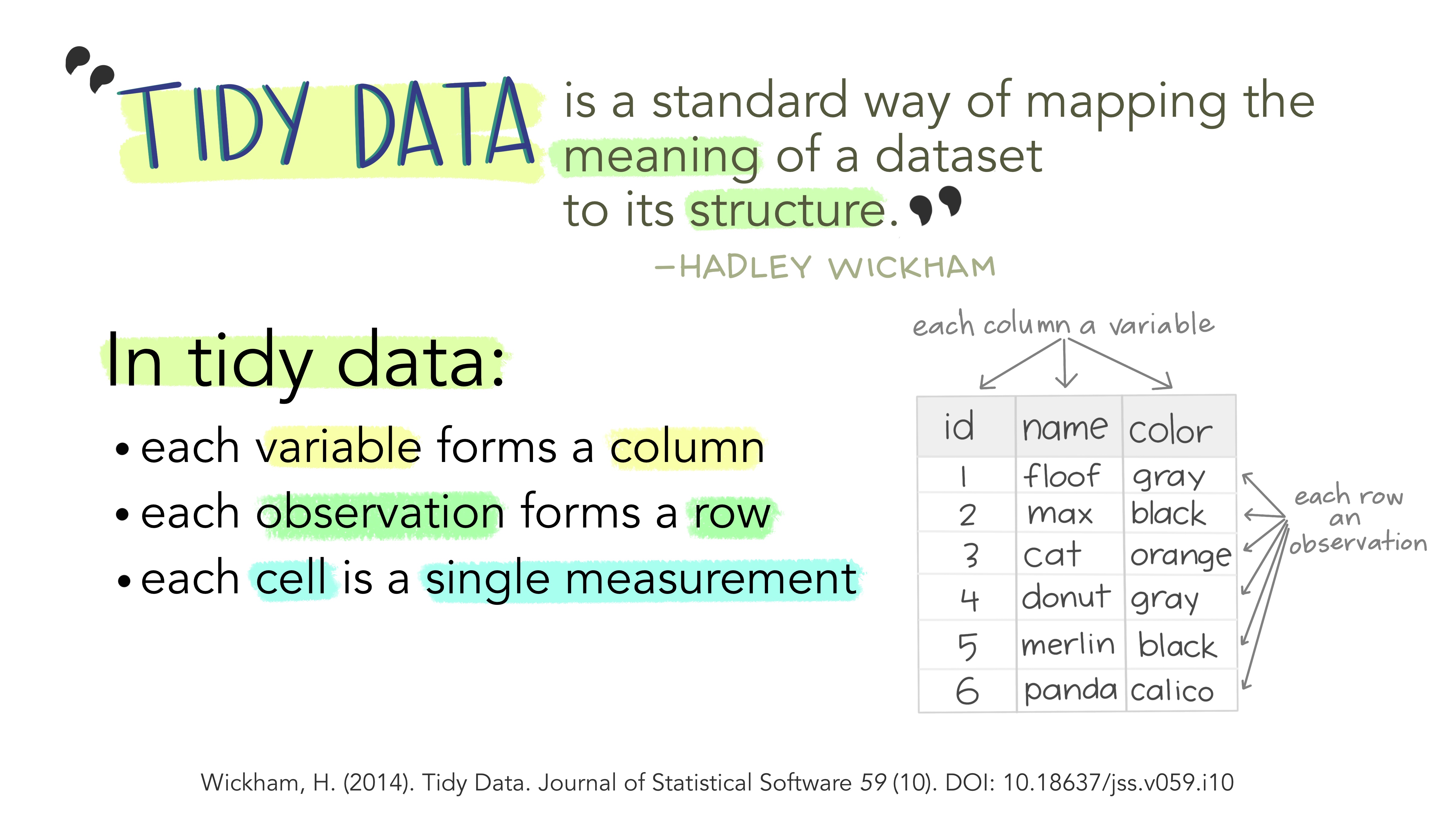
Variables
Propiedad, atributo, característica, aspecto o dimensión de un objeto, hecho o fenómeno que puede variar y cuya variación es medible.
Variables categóricas: Expresan una cualidad, característica o atributo que solo se pueden clasificar o categorizar mediante el conteo. Se establecen en rango o categorías y sólo pueden tomar los valores que únicamente pertenecen al conjunto.
Variables continuas: variables numéricas que no pueden ser contadas y tienen un número infinito de valores entre un intervalo determinado. Nunca puede ser medido con exactitud y depende de la precisión de los equipos de medida..
Data

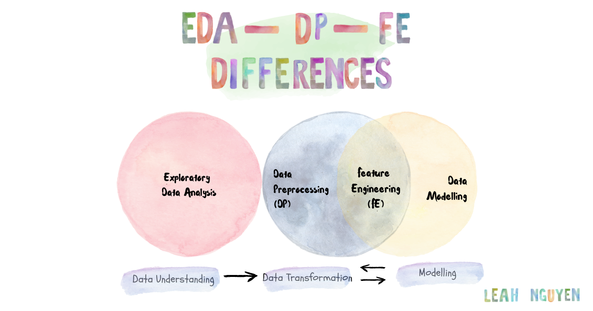
Exploratory Data Analysis (EDA)
Exploratory Data Analysis (EDA) is the very first step before you can perform any changes to the dataset or develop a statistical model to answer business problems. In other words, the process of EDA contains summarizing, visualizing and getting deeply acquainted with the important traits of a data set.
- What kind of data is this?
- How complex is this data?
- Is this data sufficient for meeting our ultimate goal
- Is there any missing data?
- Are there any missing values?
- Is there any relationship between different independent variables of the dataset? If yes then how strong is that relationship?
- Are observations independent or tightly coupled?
Data Preprocessing
Data Preprocessing is usually about data engineers getting large volumes of data from the sources — databases, object stores, data lakes, etc — and performing basic data cleaning and data wrangling preparing them for the later part, which is essentially important before modelling — feature engineering!
- If the data has html tags then remove it.
- If data contains Null values then impute it.
- If the data has some irrelevant features then drop it
- If the data has some abbreviation then replace it.
- If the data has stop words then remove it.
Feature Engineering
Feature Engineering is known as the process of transforming raw data into features that better represent the underlying problem to predictive models, resulting in improved model accuracy on unseen data.
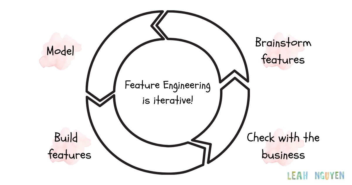
Specifically, the data scientist will begin building the models and testing to see if the features achieve the desired results. This is a repetitive process that includes running experiments with various features, as well as adding, removing, and changing features multiple times!!!
Web scraping
Web Scraping refers to the process of extracting data from a website or specific webpage. Once web scrapers extract the user’s desired data, they often also restructure the data into a more convenient format such as an csv.

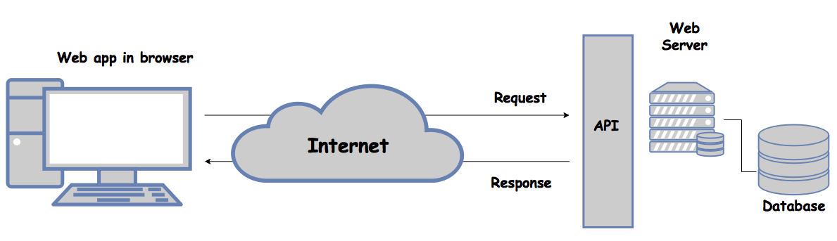
API
An API (Application Programming Interface) is a set of procedures and communication protocols that provide access to the data of an application, operating system or other services. Generally, this is done to allow the development of other applications that use the same data.
Data preprocessing

Data preprocessing

Data cleaning...The world is imperfect, so is data
- Drop multiple columns
- Change dtypes
- Encoding
- Missing data
- Remove strings in columns
- Remove white space in columns
- Concatenate two columns with strings (with condition)
- Convert timestamp(from string to datetime format)
Datos faltantes


Outliers

Outliers

Outliers

Outliers

Outliers

Escalar
Los modelos lineales o regresión logística son especialmente sensibles a este problema. Los modelos basados en arboles de decisión pueden funcionar adecuadamente sin escalar las variables.
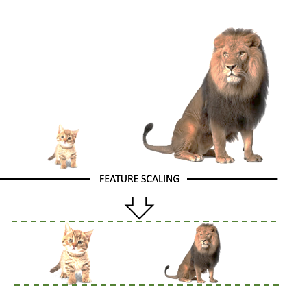
Scale invariance models
A machine learning method is 'scale invariant' if rescaling any (or all) of the features--i.e. multiplying each column by a different nonzero number--does not change its predictions.
OLS is scale invariant. If you have a model $y=w_0+w_1x_1+w_2x_2$ and you replace $x_1$ with $x'=x_1/2$ and re-estimate the model $y=w_0+2w_1x'_1+w_2x_2$, you'll get a new model which gives exactly the same preditions. The new $x'_1$ is half as big, so its coefficient is now twice as big.
When using a non-scale invariant method, if the features are of different units (e.g. dollars and miles and kilograms and numbers of products). people often standardized the data (subtract off the mean and divide by the standard deviation of each column in X.
Escalar

Escalar

Escalar

Escalar

Escalar

Binning

Label encoding

Label encoding

Clases desbalanceadas
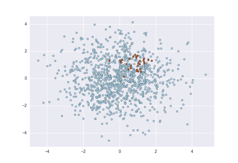
Clases desbalanceadas
- Ajuste de Parámetros del modelo: Consiste en ajustar parametros ó metricas del propio algoritmo para intentar equilibrar a la clase minoritaria penalizando a la clase mayoritaria durante el entrenamiento. Ejemplos como el parámetro class_weight = «balanced». No todos los algoritmos tienen estas posibilidades.
- Modificar el Dataset: podemos eliminar o agregar muestras de la clase mayoritaria o minoritaria para reducirlo o aumentarlo e intentar equilibrar la situación. Tiene como «peligroso» que podemos prescindir de muestras importantes, que brindan información y por lo tanto empeorar el modelo.
- Muestras artificiales: podemos intentar crear muestras sintéticas (no idénticas) utilizando diversos algoritmos que intentan seguir la tendencia del grupo minoritario. Según el método, podemos mejorar los resultados. Lo peligroso de crear muestras sintéticas es que podemos alterar la distribución «natural» de esa clase y confundir al modelo en su clasificación.
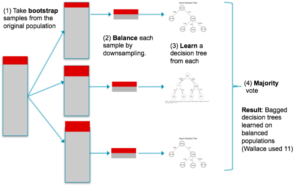
- Balanced Ensemble Methods: Utiliza las ventajas de hacer ensamble de métodos, es decir, entrenar diversos modelos y entre todos obtener el resultado final (por ejemplo «votando») pero se asegura de tomar muestras de entrenamiento equilibradas.
Clases desbalanceadas
Clases desbalanceadas

Clases desbalanceadas

Clases desbalanceadas

Frequency Distribution and Histograms
Frequency distribution table is a table that stores the categories (also called “bins”), the frequency, the relative frequency and the cumulative relative frequency of a single continuous interval variable
The frequency for a particular category or value (also called “observation”) of a variable is the number of times the category or the value appears in the dataset.
Relative frequency is the proportion (%) of the observations that belong to a category. It is used to understand how a sample or population is distributed across bins (calculated as relative frequency = frequency/n )
The cumulative relative frequency of each row is the addition of the relative frequency of this row and above. It tells us what percent of a population (observations) ranges up to this bin. The final row should be 100%.
A probability density histogram is defined so that (i) The area of each box equals the relative frequency (probability) of the corresponding bin, (ii) The total area of the histogram equals 1
Distribución de frecuencia
Distribución de frecuencia

Distribución de frecuencia
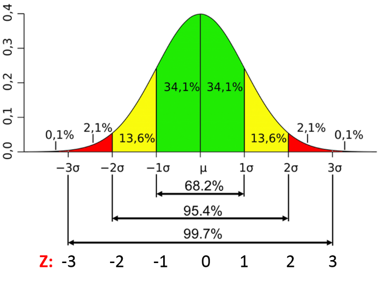
Central Limit Theorem
When we collect sufficiently large samples from a population, the means of the samples will have a normal distribution. Even if the population is not normally distributed.

Box plot
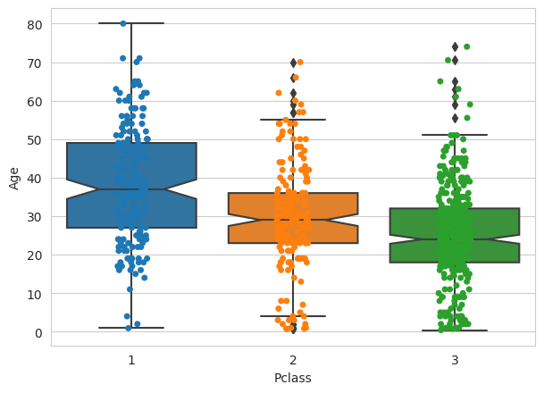
A boxplot is a graphical representation of the key descriptive statistics of a distribution.
The characteristics of a boxplot are
- The box is defined by using the lower quartile Q1 (25%; left vertical edge of the box) and the upper quartile Q3 (75%; right vertical edge of the box). The length of the box equals the interquartile range IQR = Q3 - Q1.
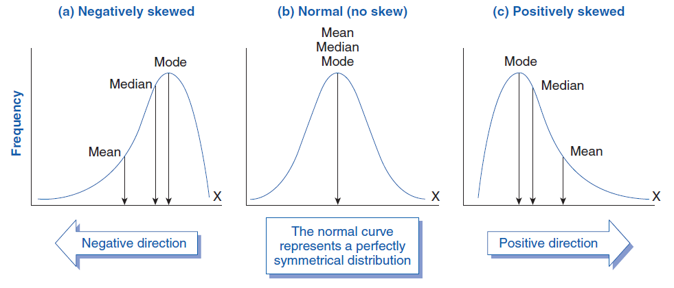
- The median is depicted by using a line inside the box. If the median is not centered, then skewness exists.
- To trace and depict outliers, we have to calculate the whiskers, which are the lines starting from the edges of the box and extending to the last object not considered an outlier.
- Objects lying further away than 1.5 IQR are considered outliers.
- Objects lying more than 3.0 IQR are considered extreme outliers, and those between (1.5 IQR and 3.0 IQR) are considered mild outliers. One may change the 1.5 or 3.0 coefficient to another value according to the study’s needs, but most statistical programs use these values by default.
- Whiskers do not necessarily stretch up to 1.5 IQR but to the last object lying before this distance from the upper or lower quartiles.


QQ plot
The normal QQ plot is a graphical technique that plots data against a theoretical normal distribution that forms a straight line
A normal QQ plot is used to identify if the data are normally distributed
If data points deviate from the straight line and curves appear (especially in the beginning or at the end of the line), the normality assumption is violated.

Scatter plot
A scatter plot displays the values of two variables as a set of point coordinates
A scatter plot is used to identify the relations between two variables and trace potential outliers.
Inspecting a scatter plot allows one to identify linear or other types of associations
If points tend to form a linear pattern, a linear relationship between variables is evident. If data points are scattered, the linear correlation is close to zero, and no association is observed between the two variables. Data points that lie further away on the x or y direction (or both) are potential outliers
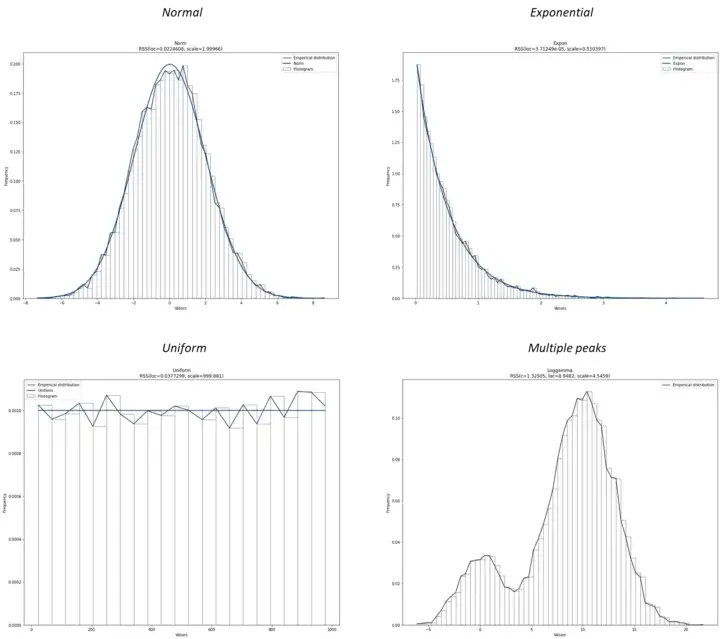
Statistical Probability Distributions
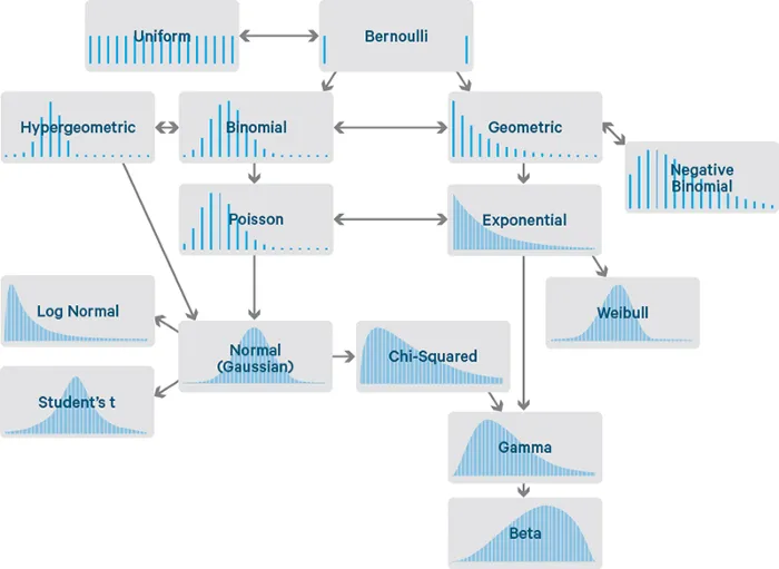
Underlying data distribution
Before making modeling decisions, you need to know the underlying data distribution.
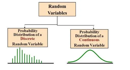
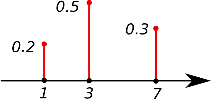
PMF: Probability Mass Function
Returns the probability that a discrete random variable X is equal to a value of x. The sum of all values is equal to 1. PMF can only be used with discrete variables.
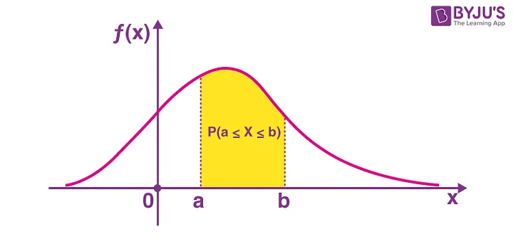
PDF: Probability Density Function
It is like the version of PMF for continuous variables. Returns the probability that a continuous random variable X is in a certain range.
CDF: Cumulative Density Function
Returns the probability that a random variable X takes values less than or equal to x.

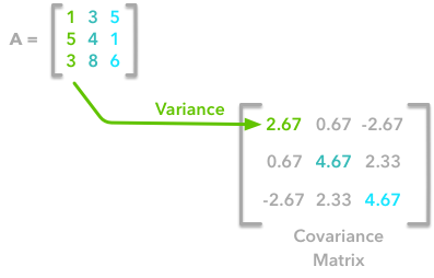
Covariance matrix
Covariance is a measure of the extent to which two variables vary together (i.e., change in the same linear direction). Covariance Cov(X, Y) is calculated as:
$cov_{x,y}=\frac{\sum_{i=1}^{n}(x_{i}-\bar{x})(y_{i}-\bar{y})}{n-1}$where $x_i$ is the score of variable X of the i-th object, $y_i$ is the score of variable Y of the i-th object, $\bar{x}$ is the mean value of variable X, $\bar{y}$ is the mean value of variable Y.
For positive covariance, if variable X increases, then variable Y increases as well. If the covariance is negative, then the variables change in the opposite way (one increases, the other decreases). Zero covariance indicates no correlation between the variables.
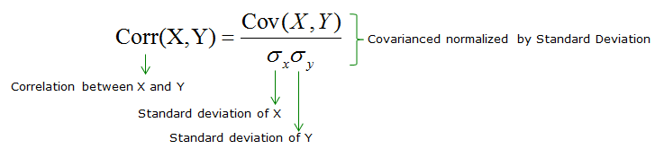
Correlation coefficient
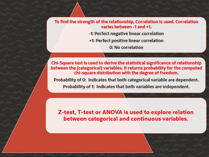
Correlation coefficient $r_{(x, y)}$ analyzes how two variables (X, Y) are linearly related. Among the correlation coefficient metrics available, the most widely used is the Pearson’s correlation coefficient (also called Pearson product-moment correlation),
$r_{(x, y)} = \frac{\text{cov}(X,Y)}{s_x s_y}$Correlation is a measure of association and not of causation.


Selección de variables

Selección de variables
Often, in a high dimensional dataset, there remain some entirely irrelevant, insignificant and unimportant features. It has been seen that the contribution of these types of features is often less towards predictive modeling as compared to the critical features. They may have zero contribution as well. These features cause a number of problems which in turn prevents the process of efficient predictive modeling.
- Unnecessary resource allocation for these features.
- These features act as a noise for which the machine learning model can perform terribly poorly.
- The machine model takes more time to get trained.
- It reduces the complexity of a model and makes it easier to interpret.
- It improves the accuracy of a model if the right subset is chosen.
- It reduces Overfitting.
Selección de variables

Feature selection & Feature transformation
Sometimes, feature selection is mistaken with dimensionality reduction. But they are different. Feature selection is different from dimensionality reduction. Both methods tend to reduce the number of attributes in the dataset, but a dimensionality reduction method does so by creating new combinations of attributes (sometimes known as feature transformation), whereas feature selection methods include and exclude attributes present in the data without changing them.
- Features Independientes: Para no tener redudancias tus features deberían ser lo más independientes posible entre ellas.
- Cantidad de Features controlada: Nuestra intuición nos falla en dimensiones superiores a 3. En la mayoría de los casos aumentar la cantidad de features afecta negativamente la performance si no contamos con una gran cantidad de datos. Por ultimo pocas features aseguran una mejor interpretabilidad de los modelos
Filter methods
Filter method relies on the general uniqueness of the data to be evaluated and pick feature subset, not including any mining algorithm. Filter method uses the exact assessment criterion which includes distance, information, dependency, and consistency.

Wrapper methods
A wrapper method needs one machine learning algorithm and uses its performance as evaluation criteria. This method searches for a feature which is best-suited for the machine learning algorithm and aims to improve the mining performance.

Embedded methods
Embedded methods are iterative in a sense that takes care of each iteration of the model training process and carefully extract those features which contribute the most to the training for a particular iteration.
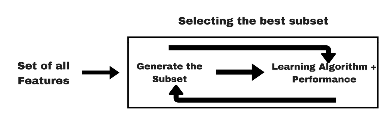
Filter vs. wrapper methods
- Filter methods do not incorporate a machine learning model in order to determine if a feature is good or bad whereas wrapper methods use a machine learning model and train it the feature to decide if it is essential or not.
- Filter methods are much faster compared to wrapper methods as they do not involve training the models. On the other hand, wrapper methods are computationally costly, and in the case of massive datasets, wrapper methods are not the most effective feature selection method to consider.
- Filter methods may fail to find the best subset of features in situations when there is not enough data to model the statistical correlation of the features, but wrapper methods can always provide the best subset of features because of their exhaustive nature.
- Using features from wrapper methods in your final machine learning model can lead to overfitting as wrapper methods already train machine learning models with the features and it affects the true power of learning. But the features from filter methods will not lead to overfitting in most of the cases
Análisis de variables
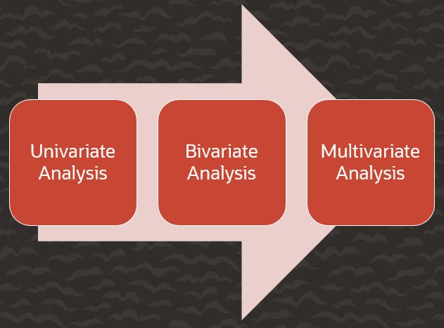
Análisis univariado

Análisis univariado
Análisis bivariado
Análisis bivariado
Independencia de las variables

Relación con la variable dependiente

Incertidumbre, desempeño & predicción

Incertidumbre
- Aleatoric Uncertainty: this is the uncertainty that is inherent in the process we are trying to explain. Uncertainty in this category tends to be irreducible in practice.
- Epistemic Uncertainty: this is the uncertainty attributed to an inadequate knowledge of the model most suited to explain the data. This uncertainty is reducible given more knowledge about the problem at hand. e.g. reduce this uncertainty by adding more parameters to the model, gather more data etc.


En teoría...


En realidad...


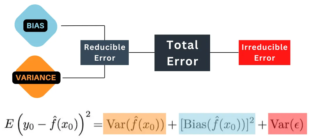
Error (error):
La diferencia entre el valor mapeado o la clase y el valor o clase verdadero

- Reducible error: $\widehat{f}$ will not be a perfect estimate for $f$ real, and this inaccuracy will introduce some error. This error is reducible because we can potentially improve the accuracy of $\widehat{f}$ by using the most appropriate statistical learning technique to estimate $f$.
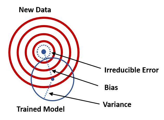
- Irreducible error: Our prediction would still have some error in it. This is because $\widehat{Y}$ is also a function of $\widehat{x}$, which, by definition, cannot be predicted using $X$. The quantity may contain unmeasured variables that are useful in predicting $Y$ : since we don’t measure them, $\widehat{f}$ cannot use them for its prediction. The quantity may also contain unmeasurable variation.


Bias - Variance trade-off
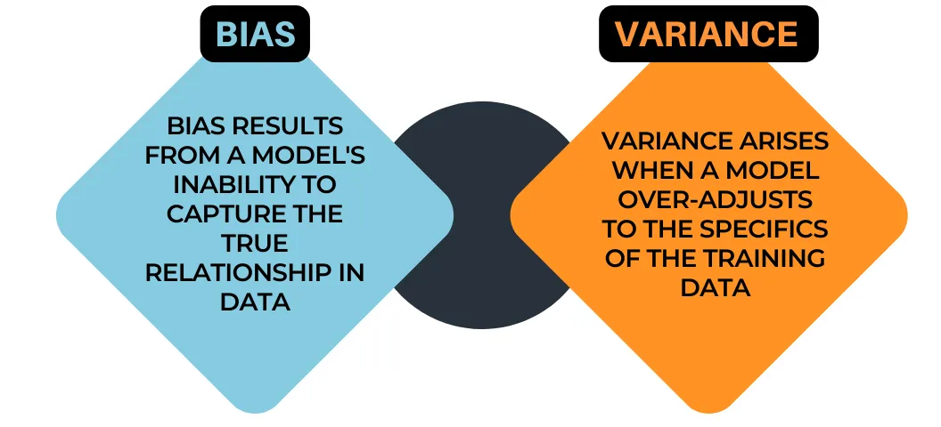
Bias: is the amount of error introduced by approximating real-world phenomena with a simplified model.
- Low Bias: Suggests less assumptions about the form of the target function.
- High Bias: Suggests more assumptions about the form of the target function.
Variance: is how much your model's test error changes based on variation in the training data. It reflects the model's sensitivity to the idiosyncrasies of the data set it was trained on.
- Low Variance: Suggests small changes to the estimate of the target function with changes to the training dataset.
- High Variance: Suggests large changes to the estimate of the target function with changes to the training dataset.


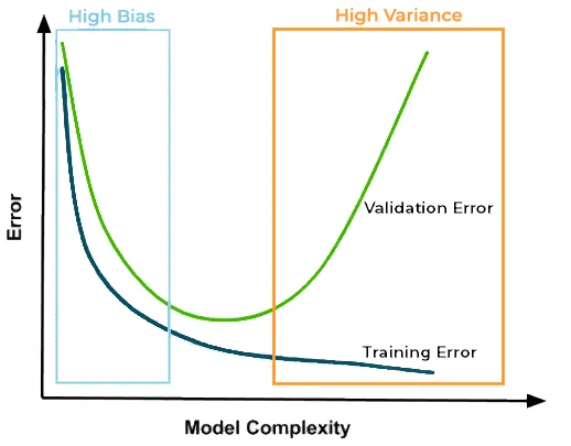
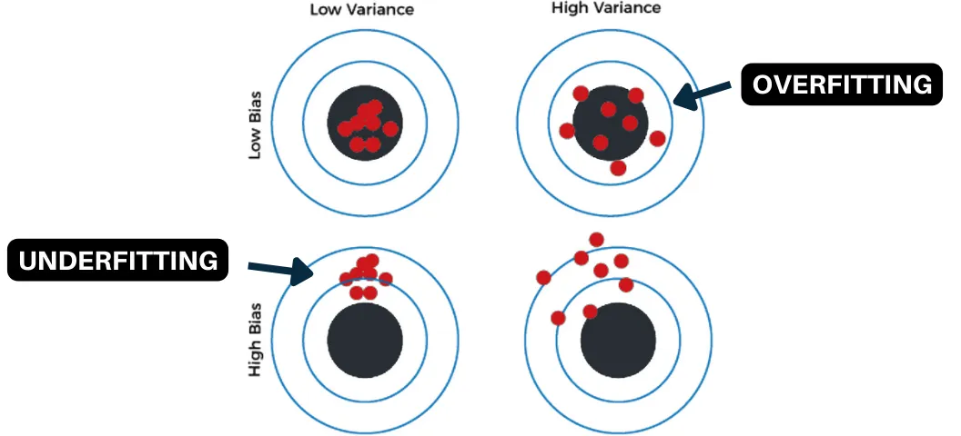
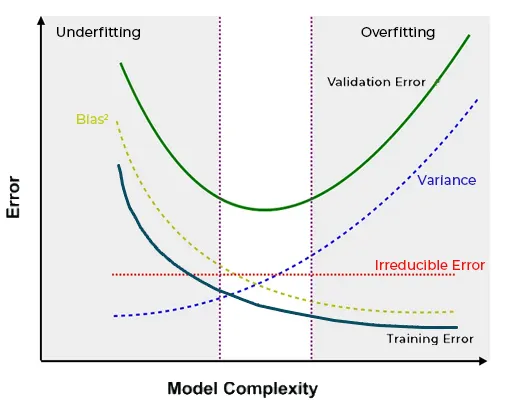


Cómo explica esta figura?

Cómo explica esta figura?

Cómo explica esta figura?

High Bias (underfitting)
- Model is too simple
- Omission of influential predictors
Indicators of High Bias
- Poor performance on both the training and test datasets
- Consistent underwhelming performance across different datasets
- Incorrect model assumptions
Techniques to Address Bias
- Using more Complex Models
- Incorporating more Features
- Reducing Regularization Strength
High Variance (overfitting)
- Model is too complex
- Capturing Noise along with the Underlying Pattern
Indicators of High Variance
- High sensitivity to changes in the training data
- Poor performance on cross-validation
- Poor performance on test data
- Model has a large number of parameters
Techniques to Address Variance
- Gathering more Training Data
- Feature Selection or Dimensionality Reduction
- Introducing Regularization
- Using Ensemble Methods
- Pruning Methods in Decision Trees
Tenga en cuenta...
- Having too many features may introduce high variance and results in overfitting.
- It is always a good idea to review the importance of features using Exploratory Data Analysis (EDA) or by using domain knowledge.
- If a feature is adding little value in predicting the dependent variable it makes sense not to use that feature.
- On the other hand, if the model is underfitting, it means that the model is not learning enough to fit sufficient number of points by finding the right hyperplane. In such a scenario, more features should be added in the model.
Number of Training Records
- Increasing the number of training records generally tends to help reduce Variance.
- However, it also depends on the quality of data. For example, if the test data has some particular type of data which is not at all present in training data then overfitting is bound to happen because the model has not learnt a particular type of data in the training. In such a case, if we just add more data records in training data but do not add the type of data which was actually missing from the training dataset earlier, then this would not help in reducing variance.
- If the model is having high bias, then adding data does not help beyond a certain point. The training error remains almost constant after certain point as we increase the number of training records.
Los datos para reducir el sobre-ajuste

Early Stopping
- Early stopping is used in Neural Network and Tree based algorithms. As shown in the graph below, in Neural networks it may happen that the difference between the training error and cross validation error reduces as the number of epochs increases. It reaches its minimum value on certain epoch and then increases in subsequent epochs. In early stopping, we stop the algorithm on the epoch (or the next epoch) showing minimum difference between train and cross validation error.
- In Decision trees, the variance increases as the depth of the tree increases. To make sure we don’t overfit, the growth of the decision tree is stopped at the optimum depth. This is typically achieved in two ways. First is stopping the tree growth if the number of data points at a node less than some specific threshold value. In this case, having too few number of data points on a sample indicate that the tree might be picking up some noisy points or outliers. The second way is to stop the growth of the tree at length which gives minimum cross validation error.

Choice of Machine Learning Algorithm:
- Bias -Variance trade-off can be controlled using regularization and other means in all machine learning algorithms. However, some ML algorithms such as Deep Neural networks, tend to overfit more. This is because, Deep Neural networks are typically used in applications having huge number of features (e.g. Computer Vision).
- Bagging (Random Forest) and Boosting (Gradient Boosted Decision Trees) are algorithms that inherently reduce Variance and Bias respectively. In Random Forest, the base learners (Decision Trees) are of higher depth which make the base learners more prone to overfitting (i.e. high variance) but because of the Randomization, the overall variance on the aggregate level reduces significantly. On the other hand, Boosting algorithms such as Gradient Boosted Decision Trees (GBDT) use shallow base learners which are more prone to underfitting (i.e. high bias) but it reduces the bias on aggregate level by sequentially adding and training simple (shallow decision trees with less complexity) base learners.
Learning curve


Validación del modelo
La evaluación de un modelo considera dos aspectos del desempeño de un modelo:
- Poder explicativo: el cual consiste en la evaluación del poder de
explicación, el cual mide la fuerza de la relación indicada por la función $f$.
- Poder predictivo: se refiere al desempeño de la función $f$ con nuevos datos.
La validación en modelos explicativos consiste de dos partes:
- validar que la función $\hat{f}$ adecuadamente representa $f$, y
- el ajuste del modelo que valida que la función f se ajuste a los datos (X,y).
La validación en modelo predictivos se enfoca en la generalización, la cual consiste en la habilidad de la función $f$ en predecir con nuevos datos (X,y).
La aceptación de un modelos debe responder al menos tres criterios:
- Su adecuación (conceptual y matemáticamente) en describir el comportamiento del sistema
- Su robustez a pequeños cambios de los parámetros de entrada (e.j. sensibilidad a los datos)
- Su exactitud en predecir los datos observados
La evaluación debe ser chequeada:
- Contra la información usada para preparar el pronóstico (Success rate). Se refiere a la “bondad del ajuste” del modelo. Qué tan bien el modelo se desempeña?
- Contra el futuro, cuando el evento finalmente ocurra (Prediction rate). Se refiere a la habilidad del modelo para predecir adecuadamente los futuros deslizamientos. Qué tan bien el modelo predice?
En general es mas fácil obtener niveles altos del ajuste del modelo que alcanzar niveles similares para el desempeño de la predicción. Y sin embargo el segundo es mas importante para efectos prácticos.
Cross validation

Cross validation

Train-test-split

Train-test-split

Train-test-split

k-fold

k-fold

k-fold

leave-one-out

Stratified kfold

Métrica para Regresión
Mean Absolute Error (MAE):
If the absolute value is not taken (the signs of the errors are not removed), the average error becomes the Mean Bias Error (MBE) and is usually intended to measure average model bias. MBE can convey useful information, but should be interpreted cautiously because positive and negative errors will cancel out.
Root Mean Squared Error (RMSE):
- Both metrics can range from 0 to ∞ and are indifferent to the direction of errors.
- They are negatively-oriented scores, which means lower values are better.
R-squared ($R^2$):
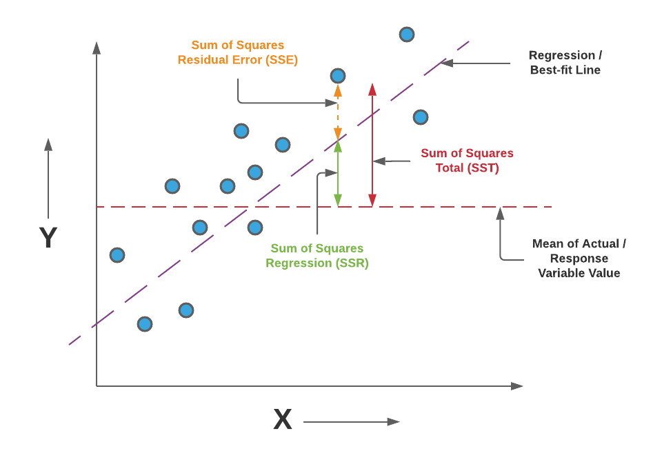
R-squared ($R^2$):

R-squared ($R^2$) is a statistical measure that represents the proportion of the variance for a dependent variable that's explained by an independent variable or variables in a regression model.
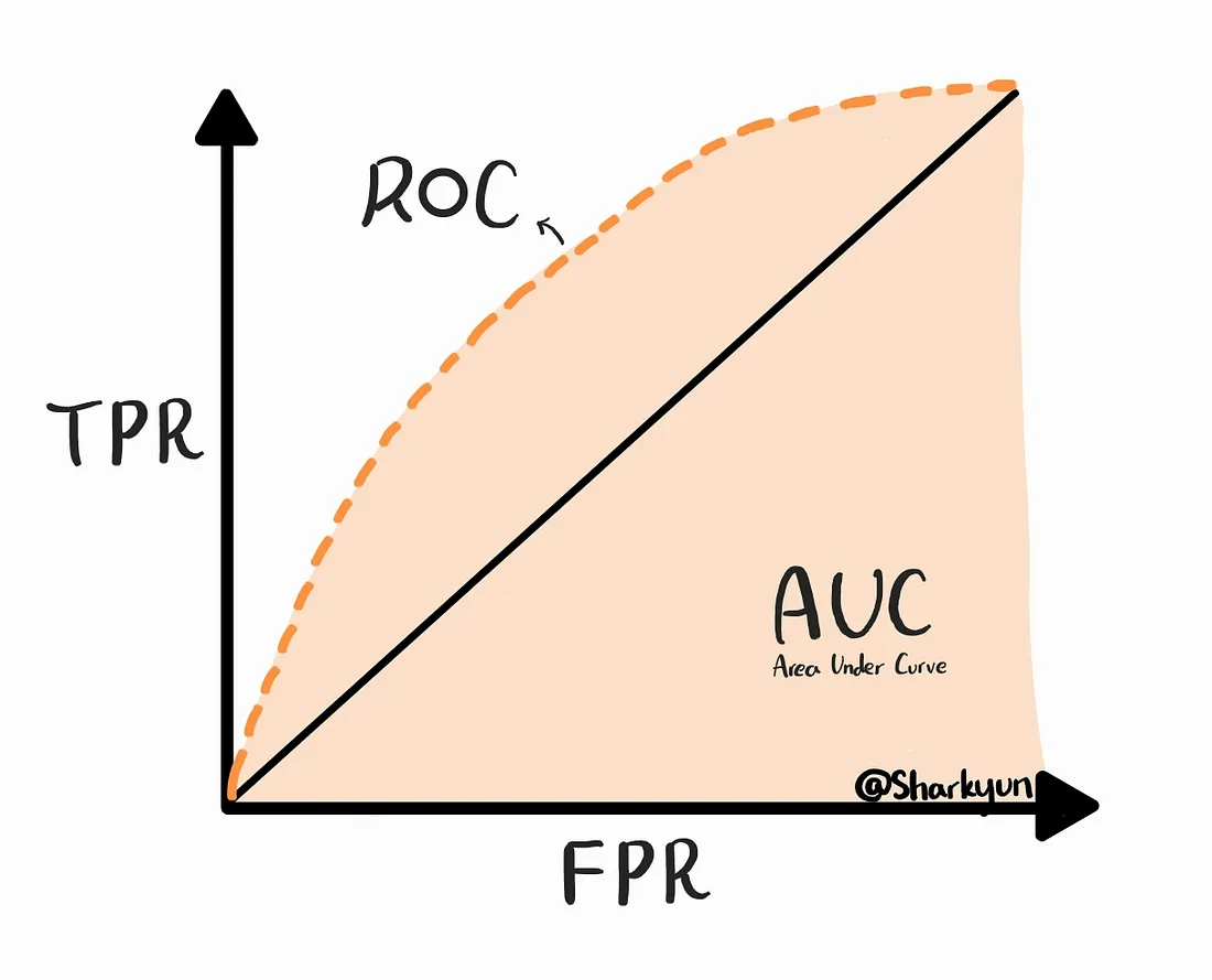
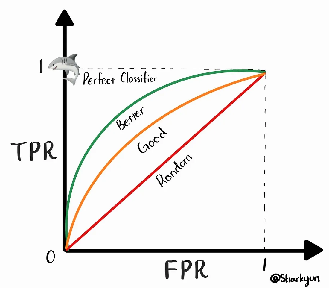
Métrica para Clasificación
Matriz de confusión


Statistical Inference
Statistical inference
process of analyzing sample data and making conclusions about the parameters of a population is called Statistical Inference
There are three common forms of Statistical Inference. Each one has a different way of using sample data to make conclusions about the population. They are:
- Point Estimation
- Interval Estimation
- Hypothesis Testing
Point stimation
For Point Estimate, we infer an unknown population parameter using a single value based on the sample data.
If we took another set of sample data (with the same sample size) and do a point estimate again, it is very likely we would end up making a different conclusion about the population. That means there is uncertainty when we draw conclusions about the population based on the sample data. Point estimation doesn’t give us any idea as to how good the estimation is.
Interval stimation
For Interval Estimation, we use an interval of values (aka Confidence Interval) to estimate an unknown population parameter, and state how confident we are that this interval would include the true population parameter.
To construct the confidence interval, we would need two metrics:
- the point estimate of the population parameter (e.g., sample mean)
- the standard error of the point estimate (e.g., the standard error of the sample mean), which indicates how different the population parameter is likely to be from one sample statistic.
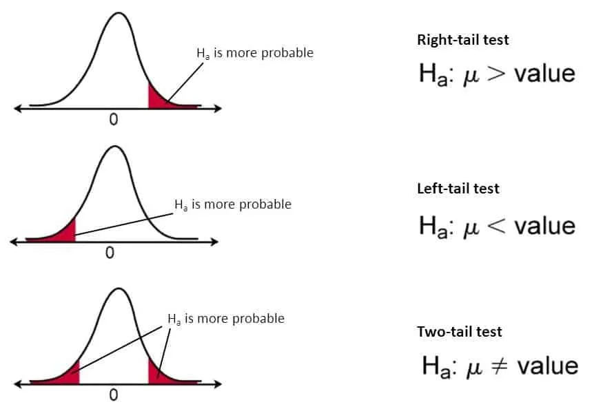
Hypothesis Testing
In statistics, when we have collected data from experiments, surveys, or observations, we often want to determine if the observed differences or effects (i.e., x̄ - µ) are statistically significant or just the result of random chance.
Once the test statistic (Z statistic or T statistic) is calculated, we determine the critical region — the region of extreme values that would lead us to reject the null hypothesis. This critical region is established based on the chosen significance level (alpha), which represents the probability of making a Type I error (rejecting the null hypothesis when it is true). Common significance levels include 0.05 (5%) or 0.01 (1%).
If the calculated test statistic falls within the critical region, we reject the null hypothesis in favor of the alternative hypothesis, suggesting that the observed sample results are statistically significant.
P-value

Hypothesis testing
Unlike point estimate and interval estimate which are used to infer population parameters based on sample data, the purpose of hypothesis testing is to evaluate the strength of evidence from the sample data for making conclusions about the population
In a hypothesis test, we evaluate two mutually exclusive statements about the population. They are
- Null Hypothesis (H0)
- Alternative Hypothesis (Ha)
Note: A hypothesis test is NOT designed to prove the null or alternative hypothesis. Instead, it evaluates the strength of evidence AGAINST the null hypothesis using sample data. If a p-value is less than the Significance Level. That means the evidence (against the null hypothesis) we found from the sample data would rarely occur by chance. Therefore, We have enough evidence to reject the null hypothesis. It doesn’t mean we’ve proved the alternative hypothesis is correct. It only means we accept the alternative hypothesis or we’re more confident that the alternative hypothesis is correct.
Hypothesis Testing
We describe a finding as statistically significant by interpreting the p-value.
A statistical hypothesis test may return a value called p or the p-value. This is a quantity that we can use to interpret or quantify the result of the test and either reject or fail to reject the null hypothesis. This is done by comparing the p-value to a threshold value chosen beforehand called the significance level.
A common value used for alpha is 5% or 0.05. A smaller alpha value suggests a more robust interpretation of the null hypothesis, such as 1% or 0.1%.
- If p-value > alpha: Fail to reject the null hypothesis (i.e. not significant result).
- If p-value <= alpha: Reject the null hypothesis (i.e. significant result).
Hypothesis Testing
On a very broad level if we have prior knowledge about the under lying data distribution (mainly normal distribution) then parametric tests like T-Test, Z-Test, ANOVA test etc are used. And if we don’t have prior knowledge about the underlying data distribution then non-parametric tests like Mann-Whitney U Test is used.
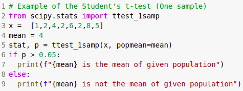
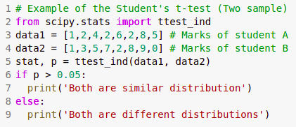
T-Test
It is used for hypothesis testing mainly when sample size is very less (less than 30) and sample standard deviation is not available. However under lying distribution is assumed to be normal. A T-Test is of two types. One-Sample T-Test, which is used for comparing sample mean with that of a population mean. Two-Sample T-Test, which is used for comparing means of two samples. When observation across each sample are paired then it is called Pared T-Test.
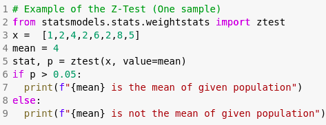
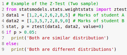
Z-Test
It is used for hypothesis testing mainly when sample size is high (greater than 30) . And under lying distribution is assumed to be normal. A Z-Test is of two types. One-Sample Z-Test, which is used for comparing sample mean with that of a population mean. Two-Sample Z-Test, which is used for comparing means of two samples.
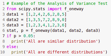
ANOVA Test
ANOVA Test stands for Analysis of Variance. It is a generalisation or extension for Z-Test. This test tells us whether two or more samples are significantly same or different. Similar to Paired T-Test, there is also Repeated Measures ANOVA Test which tests whether the means of two or more paired samples are significantly different or not.
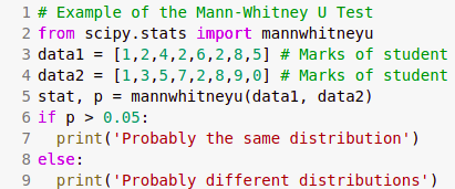
Non-Parametric tests
When we have prior knowledge of underlying data distribution (gaussian distribution), then parametric tests are carried out. Some of the non-parametric test are as follows
- Mann-Whitney U Test
- Wilcoxon Signed-Rank Test
- Kruskal-Wallis H Test
- Friedman Test
Hiperparámetros & Optimización
Función de optimización
Gradually, with the help of some optimization function, loss function learns to reduce the error in prediction. An optimization algorithm is a procedure which is executed iteratively by comparing various solutions until an optimum or a satisfactory solution is found. ... these algorithms minimize or maximize a Loss function using its gradient values with respect to the parameters.

The case for lineal regression
$\hat{y}=\theta_0x_0+\theta_1x_1+\theta_2x_2+\theta_3x_3+\theta_nx_n$ $\hat{y}=h(\theta)=\theta^{T}x$Loss function --» Cost function --» Optimizer
$MSE(\theta)=Cost(\theta)=J(\theta)--»min Cost(\theta)$ $J(\theta_0,\theta_1,\theta_2,...,\theta_m)=\frac{1}{2m}\sum_{i=1}^{m}(h_{\theta}(x^{(i)})-y^{(i)})^2$$θ$ → The parameters that minimize the loss function
$x$ → The input feature values
$y$ → The vector of output values
$\hat{y}$ → The vector of estimated output values
$h(\theta)$ → the hypothesis function
The Normal equation
In a linear regression problem, optimizing a model can be done by using a mathematical formula called the Normal Equation.
$\theta=(X^T X)^{-1} X^Ty$It is as a one-step algorithm used to analytically find the coefficients that minimize the loss function ($\theta$) without having to iterate
However, this method becomes an issue when you have a lot of data : either too much features (calculation time issue) or too much observations (memory issue).
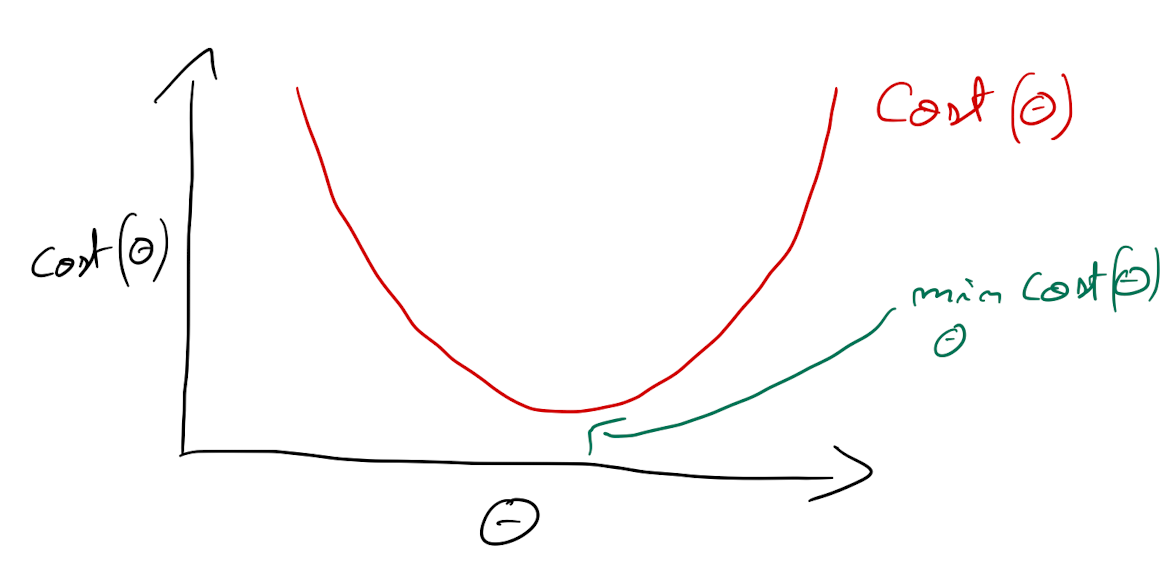
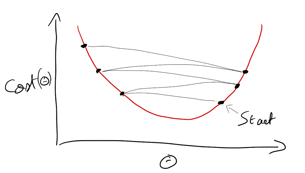
Gradiente descendente
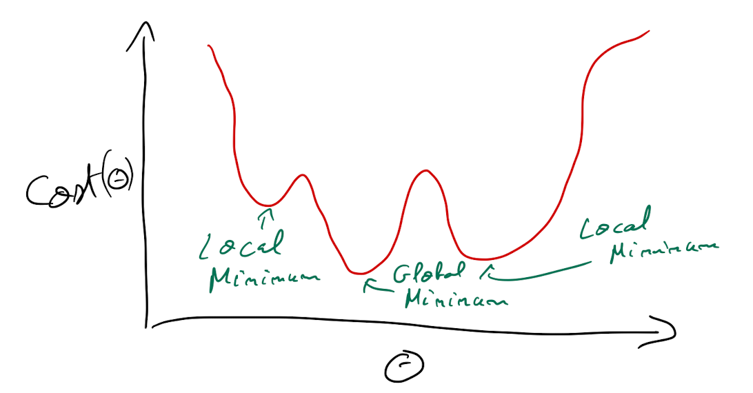
It is an optimization algorithm to find the minimum of a function. We start with a random point on the function and move in the negative direction of the gradient of the function to reach the local/global minima.
Gradiente descendente
$\frac{\partial{}}{{\partial{\theta_j}}} cost(\theta)$

Mínimo local
Learning step
Alpha (α) is called the learning rate and specify the magnitude of the steps. The higher α is, the bigger the steps are going to be and vice versa.
$\theta^{(next_step)}=\theta - \alpha \nabla_\theta cost(\theta)$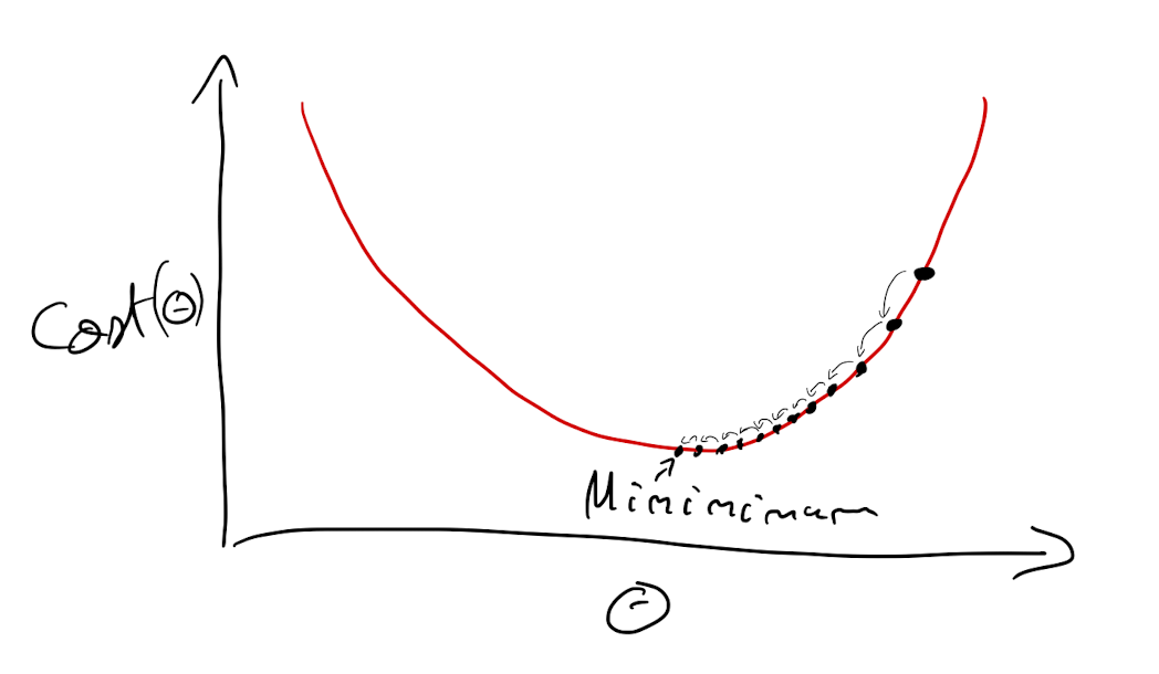
Learning step
Procedimiento manual


Procedimiento interativo


Ejemplo

Stochastic gradient descent

Selección de hiperparámetros

Selección de hiperparámetros

Selección de hiperparámetros
Selección de hiperparámetros

Selección de hiperparámetros

Selección de hiperparámetros
L1 Loss function

L2 Loss function

Huber function

Log loss
Clustering
Clustering
Definición
El objetivo es identificar subgrupos en los datos, de tal forma que los datos en cada subgrupo (clusters) sean muy similares, mientras que los datos en diferentes subgrupos sean muy diferentes.


Distancias


Tipos de clustering
- Hierarchical Clustering: descomposición jerárquica utilizando algún criterio, pueden ser aglomerativos (bottom-up) o de separación (top-down). No necesitan K al inicio.
- Partitioning Methods ( (k-means, PAM, CLARA): se construye a partir de particiones, las cuales son evaluadas por algún criterio. Necesitan K al inicio.
- Density-Based Clustering: basados en funciones de conectividad y funciones de densidad.
- Model-based Clustering: se utiliza un modelo para agrupar los modelos.
- Fuzzy Clustering: A partir de lógica difusa se separan o agrupan los clusters.

Hierarchical clustering

K-Means


Hierarchical clustering


Métrica de evaluación

Método Elbow

Método Silhouette

Método Silhouette

Método Silhouette

Método Silhouette

Método Silhouette

Método Silhouette

Consideraciones


Reduccion de dimensiones
Dimensionalidad

Dimensionalidad

Dimensionalidad

Hughes phenomenon

As the dimensions increase the volume of the space increases so fast that the available data becomes sparse
Hughes phenomenon
One more weird problem that arises with high dimensional data is that distance-based algorithms tend to perform very poorly. This happens because distances mean nothing in high dimensional space. As the dimensions increase, all the points become equidistant from each other such that the difference between the minimum and maximum distance between two points tends to zero.

Dimensionalidad

Dimensionalidad

Reducción de la dimensionalidad
Dimensionality reduction techniques can be classified in two major approaches as follows.
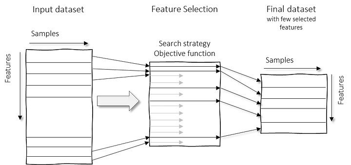
- Feature Selection methods: Specific features are selected for each data sample from the original list of features and other features are discarded. No new features are generated in this process.
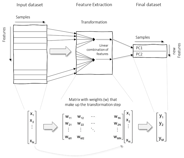
- Feature Extraction methods: We engineer or extract new features from the original list of features in the data. Thus the reduced subset of features will contain newly generated features that were not part of the original feature set. PCA falls under this category
Feature selection
Feature extraction
Componentes principales

Componentes principales

Componentes principales

Componentes principales

Componentes principales

Componentes principales

Procedimiento

Procedimiento

Procedimiento

Procedimiento

Procedimiento

Representación

Representación

Representación

Representación

Representación

Representación

Representación

Limitaciones

Limitaciones

Limitaciones

Limitaciones

Análisis Discriminante Lineal (LDA)


Análisis Discriminante Lineal (LDA)
Método supervisado que trabaja con datos que ya han sido clasificados en grupos para encontrar reglas que permitan clasificar elementos individuales nuevos no clasificados. La técnica mas conocida y utilizada se denomina Análisis de la Función Linear Discriminante de Fisher (Fisher, 1936).
- Permite clasificar a los individuos o casos (en este caso celdas o unidades de análisis) en alguno de los grupos establecidos por la variable.
- Variables canónicas o discriminantes : combinaciones lineales de las variables originales y se expresan por una Función discriminante.
- No tiene hiperparámetros
- Es muy similar al análisis de cluster, pero en este caso se cuenta con las clases a las cuales pertenece (labels), sin embargo utiliza el mismo algoritmo de PCA. Por lo que también se puede decir que es el mismo PCA pero arroja resultados similares en su forma a clúster (grupos homogéneos entre si pero heterogéneos respecto a los demás grupos) por lo que tienen una finalidad también descriptiva (identificar la variable que mejor discriminen y caracterizan a los grupos).


Procedimiento
Se pretende encontrar relaciones lineales entre las variables continuas que mejor discriminen entre grupos, para esto se realiza:
Procedimiento

Procedimiento

Procedimiento

Procedimiento


Ejemplo

Ejemplo

Ejemplo

Regresión lineal
Regresion lineal

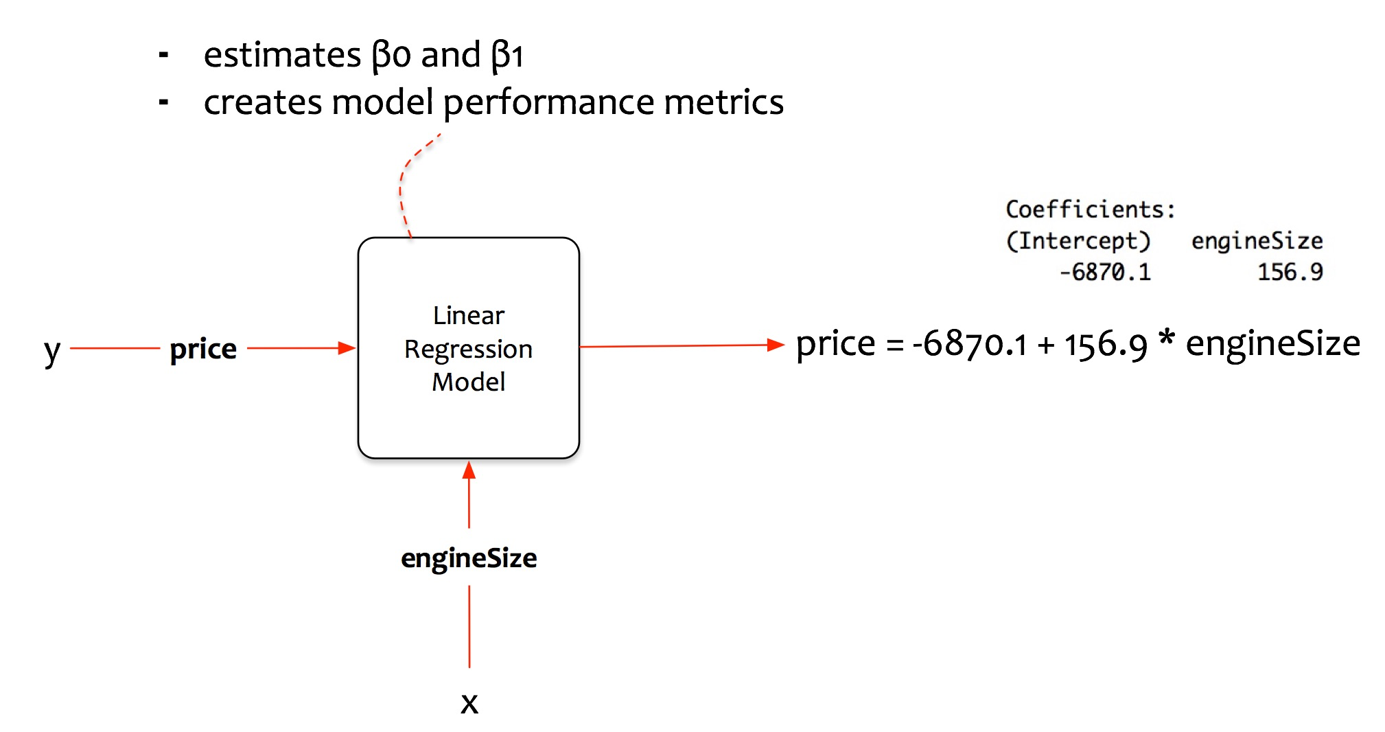
Regresión lineal univariada

Regresión lineal
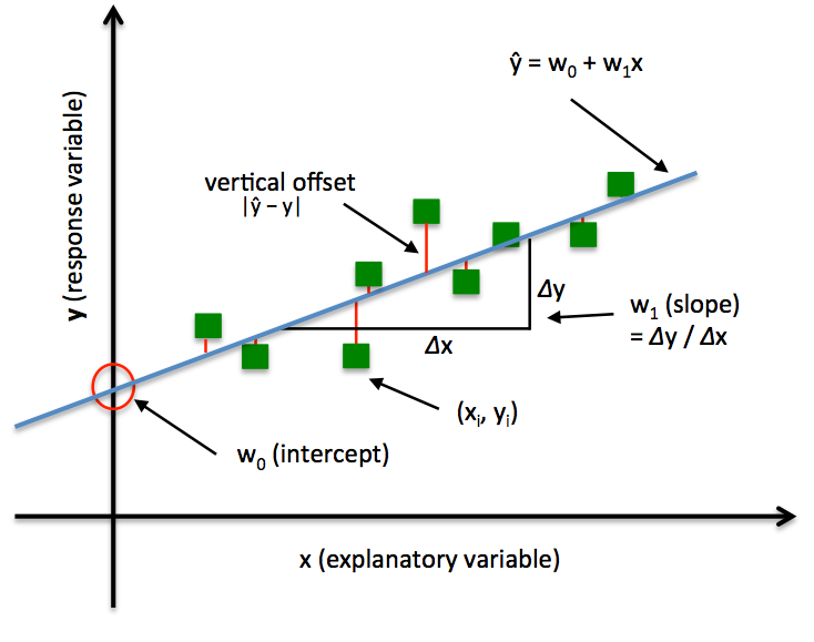
Simple Linear Regression model
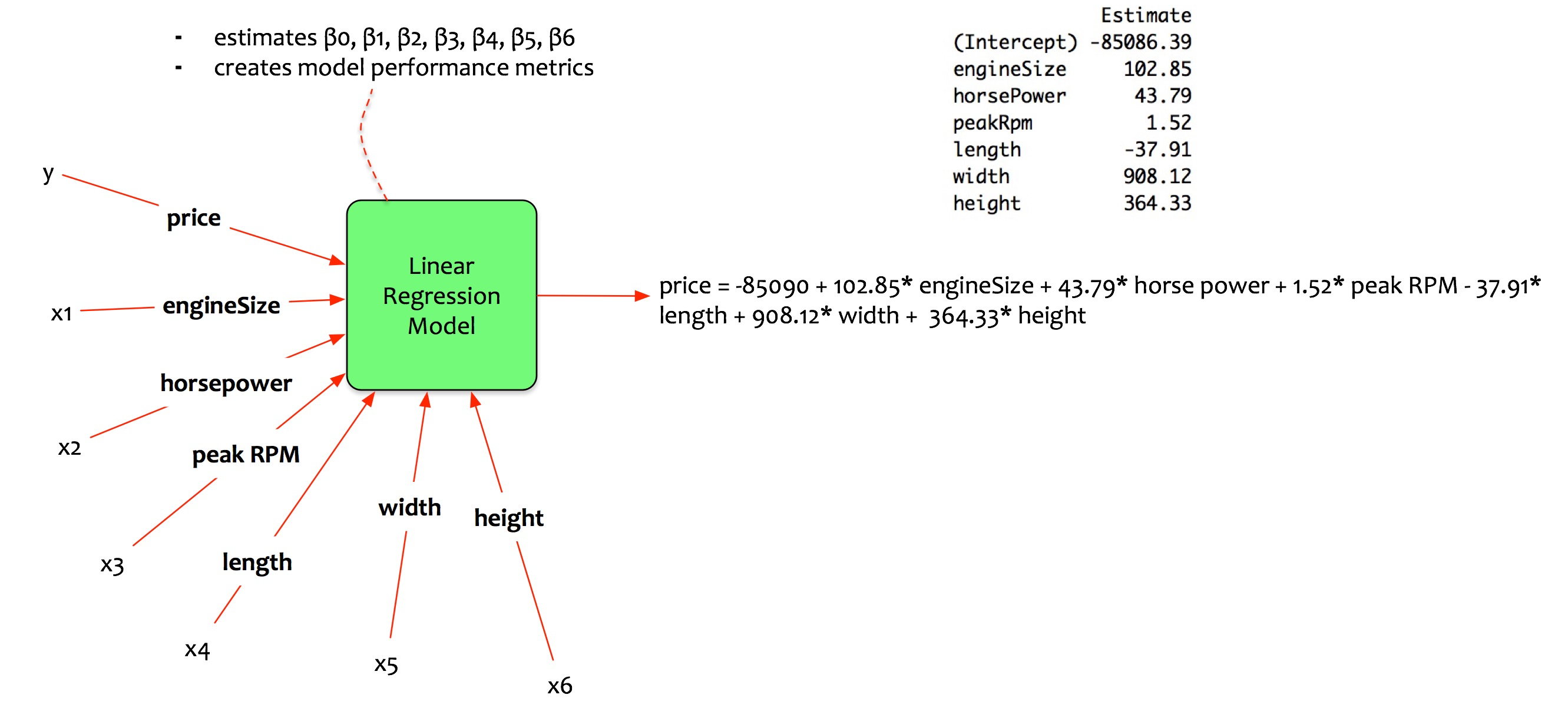
Regresión lineal multivariada

Multivariate regression model
Modelos lineales
Los siguientes son modelos lineales:
Los modelos siguen siendo lineales, ya que los coeficientes/pesos asociados con cada variable siguen siendo lineales. Se puede decir que el modelo es no linear en término de las variables, pero lineal en término de los coeficientes.En el caso del segundo modelo $y$ es función tanto de $x$ como de $x^2$. Para el tercer modelo $y$ es función tanto de $x_1$ y $x_2$ como de la interacción entre $x_1$ y $x_2$.
Modelo lineal

Modelo no lineal en términos de las variables

Intercepto
Paradoxically, while the value is generally meaningless, it is crucial to include the constant term in most regression models!...If all of the predictors can’t be zero, it is impossible to interpret the value of the constant. Don't even try!...
The constant term is in part estimated by the omission of predictors from a regression analysis. In essence, it serves as a garbage bin for any bias that is not accounted for by the terms in the model.
Estandarizar las variables
You should standardize the variables when your regression model contains polynomial terms or interaction terms. While these types of terms can provide extremely important information about the relationship between the response and predictor variables, they also produce excessive amounts of multicollinearity. Multicollinearity is a problem because it can hide statistically significant terms, cause the coefficients to switch signs, and make it more difficult to specify the correct model.
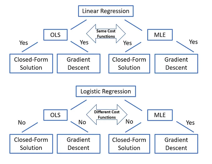
OLS & MLE estimators
Multicollinearity
Collinearity is a linear association between two explanatory variables:
Multicollinearity is a linear associations between more than two explanatory variables:
The effect of multicollinearity (redundancy) is that it makes the estimation of model parameters impossible.
To derive the ordinary least squares (OLS) estimators r must be invertible, which means the matrix must have full rank. If the matrix is rank deficient then the OLS estimator does not exist because the matrix cannot be inverted. If your design matrix contains k independent explanatory variables, then rank(r) should equal k. The effect of perfect multicollinearity is to reduce the rank of r less than the maximum number of columns.
Variance inflation factor (VIF)
VIF which quantifies the severity of multicollinearity in a multiple regression model. Functionally, it measures the increase in the variance of an estimated coefficient when collinearity is present
The coefficient of determination is derived from the regression of covariate j against the remaining k — 1 variables. If the VIF is close to one this implies that covariate j is linearly independent of all other variables. Values greater than one are indicative of some degree of multicollinearity, whereas values between one and five are considered to exhibit mild to moderate multicollinearity. these variables may be left in the model, though some caution is required when interpreting their coefficients. If the VIF is greater than five this suggests moderate to high multicollinearity, you might want to consider leaving these variables out.
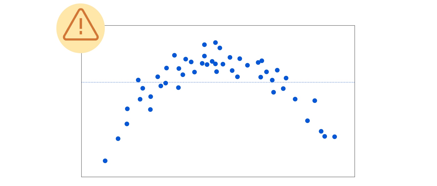
The assumptions
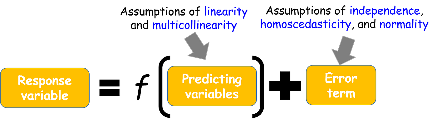
The assumptions
- Linear relationship between the dependent and independent variables
- Multivariate normality: the residual of the linear model should be normally distributed
- No multicolinearity between independent variables, i.e. they should not correlate between each other
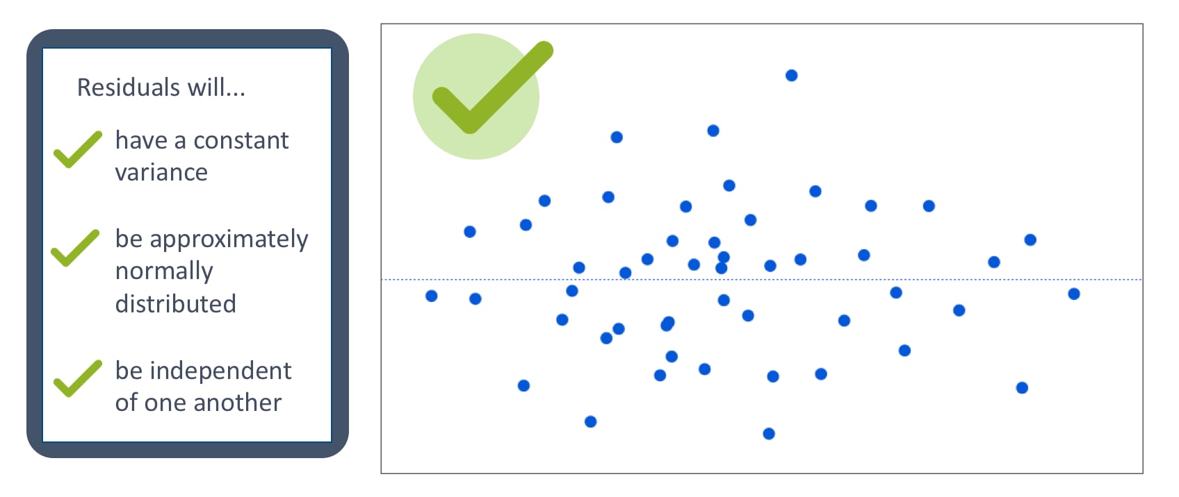
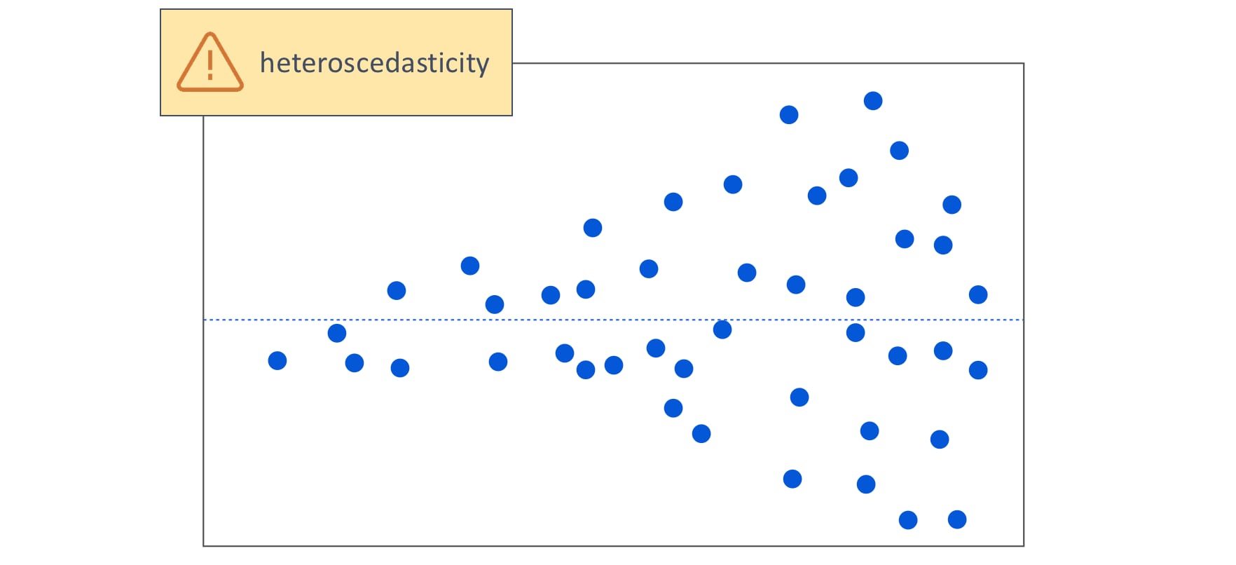
- Homoscedasticity: the errors/residuals should have constant variance (no trends)
- No autocorrelation: residuals (errors) in the model shoul not be correlqated in any way
The assumptions
The assumptions
The assumptions
The assumptions
The assumptions
Transformation
Logarithmic transformations are useful in various situations, including:
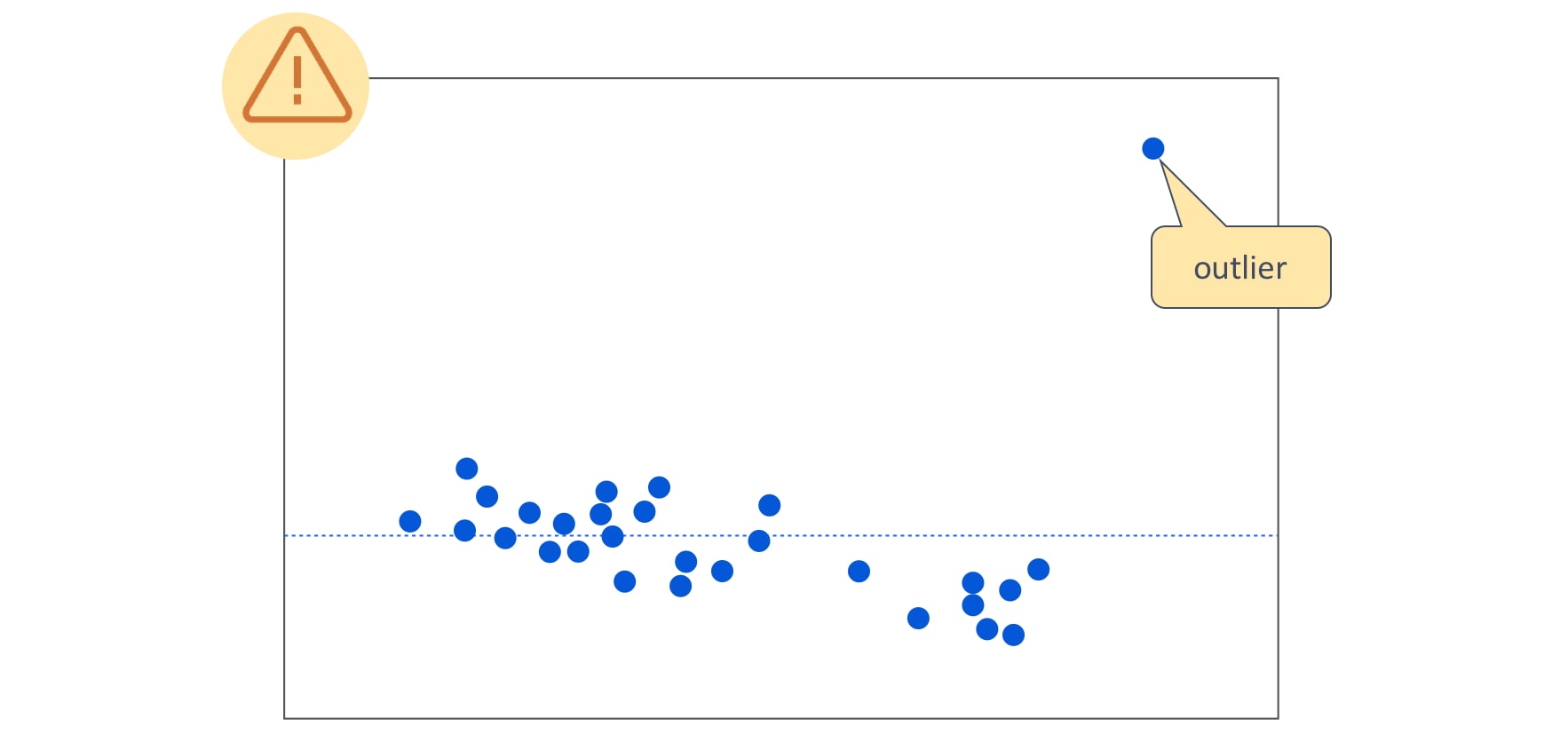
- Reducing the impact of outliers
- Transforming skewed data to approximate normality
- Linearizing relationships between variables
- Stabilizing variance in heteroscedastic data
- Simplifying complex relationships
Before applying a logarithmic transformation, it’s essential to consider the following:
- Ensure that all data values are positive, as the logarithm of zero or negative numbers is undefined.
- If necessary, add a constant to all data points to make them positive.
- Choose an appropriate logarithm base for your analysis.
Note: When interpreting results after applying a logarithmic transformation, keep in mind that the transformation has changed the scale of the data. To make meaningful interpretations, you may need to back-transform the results to the original scale.
$R^2$

Adjusted $R^2$

Resultados

Coef & t
The importance of a feature in a linear regression model can be measured by the absolute value of its t-statistic. The t-statistic is the estimated weight scaled with its standard error.
Let us examine what this formula tells us: The importance of a feature increases with increasing weight. This makes sense. The more variance the estimated weight has (= the less certain we are about the correct value), the less important the feature is. This also makes sense.
Cost function

Regularización

Regularización
A standard least squares model tends to have some variance in it, i.e. this model won’t generalize well for a data set different than its training data. Regularization, significantly reduces the variance of the model, without substantial increase in its bias
So the tuning parameter λ, used in the regularization techniques controls the impact on bias and variance. As the value of λ rises, it reduces the value of coefficients and thus reducing the variance. Till a point, this increase in λ is beneficial as it is only reducing the variance (hence avoiding overfitting), without loosing any important properties in the data.
But after certain value, the model starts loosing important properties, giving rise to bias in the model and thus underfitting. Therefore, the value of λ should be carefully selected.
Penalized linear regression
Regularization will help select a midpoint between the first scenario of high bias and the later scenario of high variance


Ridge (L1)

Lasso (L2)


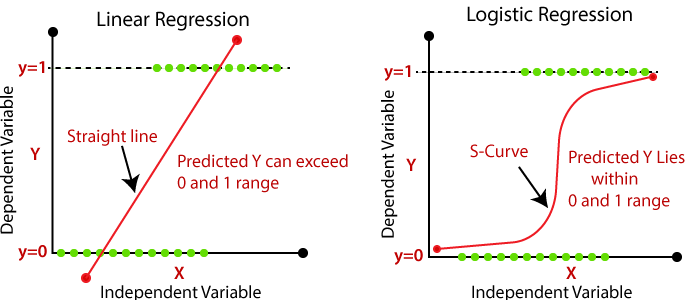
Regresión logística
Regresión logística
Regresión logística

Regresión logística

Regresión logística

Regresión logística

Regresión logística

Regresión logística

Regresión Logística
La Regresión Logística es una combinación lineal de variables independientes (factores explicativos) para explicar la varianza en una variable dependiente (inventario de deslizamientos) tipo dummy [0 – 1].
Ventajas
- Las variables predictoras pueden ser continuas, discretas, dicótomas, o cualquier combinación de ellas.
- La variable dependiente es dicotoma (binaria)
- A pesar de que el modelo transformado es lineal en las variables, las probabilidades no son lineales
Desventajas
- Los pesos de las variables terminan siendo un promedio para toda el área de estudio, los cuales en realidad pueden diferir en diferentes partes del área de estudio.
- La función objetivo es una combinacion lineal de las variables independientes
Función LOGIT

Función LOGIT

Función LOGIT
Sea p(x) la probabilidad de éxito cuando el valor de la variable predictora es x, entonces:
$p(x) = \frac{e^{a+\sum bx}}{1+e^{a+\sum bx}} = \frac{1}{1+e^{-(a+\sum bx)}}$ $\frac{p(x)}{1-p(x)} = e^{a+\sum bx}$Odds

Limitaciones de los Odds

Limitaciones de los Odds

Función LOGIT
$Ln(\frac{p(x)}{1-p(x)}) = a+\sum bx$Donde $a$ es el intercepto del modelo, $b$ son los coeficientes del modelo de regresión logística, y $x$ son las variables independientes (predictoras).
$P(y=1) = \frac{1}{1+e^{-(a+\sum bx)}}$Donde, P es la probabilidad de Bernoulli que una unidad de terreno pertenece al grupo de no deslizamientos o al grupo de si deslizamiento. P varía de 0 a 1 en forma de curva “S” (logística).
Odds

Regresión Logística

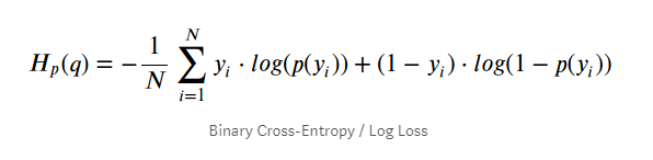
Función de costo
En regresión logística no se puede utilizar el estimador OLS, ya que en este caso no tiene una solución analítica y no se puede utilizar gradiente descendente por que no es una función convexa. En su defecto, se utiliza MLE y Binary cross-entropy.

Función de costo

Regresión Logística

Regresión Logística

Regresión Logística

										LogisticRegression(X, y,
											pos_class=None,
											Cs=10,
											fit_intercept=True,
											max_iter=100,
											tol=1e-4,
											verbose=0,
											solver='lbfgs',
											coef=None,
											class_weight=None,
											dual=False, penalty='l2',
											intercept_scaling=1.,
											multi_class='auto',
											random_state=None, check_input=True,
											max_squared_sum=None,
											sample_weight=None,
											l1_ratio=None):
Hiperparámetro C

KNN
KNN
Utiliza todo el dataset para entrenar cada punto y por eso requiere de uso de mucha memoria y recursos de procesamiento (CPU). Por estas razones KNN tiende a funcionar mejor en datasets pequeños y sin una cantidad enorme de features (las columnas).

KNN
Brute force search

KNN
Lazy learning: KNN no genera un modelo fruto del aprendizaje con datos de entrenamiento, sino que el aprendizaje sucede en el mismo momento en el que se prueban los datos de test.
Basado en Instancia: Esto quiere decir que nuestro algoritmo no aprende explícitamente un modelo (como por ejemplo en Regresión Logística o árboles de decisión). En cambio memoriza las instancias de entrenamiento que son usadas como base de conocimiento para la fase de predicción.
Modelo supervisado: A diferencia de K-means, que es un algoritmo no supervisado y donde la «K» significa la cantidad de grupos (clusters) que deseamos clasificar, en K-Nearest Neighbor la «K» significa la cantidad de «puntos vecinos» que tenemos en cuenta en las cercanías para clasificar los «n» grupos -que ya se conocen de antemano, pues es un algoritmo supervisado.
Nonparametric: KNN makes no assumptions about the functional form of the problem being solved. As such KNN is referred to as a nonparametric machine learning algorithm.

KNN

KNN

KNN

KNN
- λ = 1 is the Manhattan distance. Synonyms are L1-Norm, Taxicab or City-Block distance. For two vectors of ranked ordinal variables, the Manhattan distance is sometimes called Foot-ruler distance.
- λ = 2 is the Euclidean distance. Synonyms are L2-Norm or Ruler distance. For two vectors of ranked ordinal variables, the Euclidean distance is sometimes called Spearman distance.
- λ = ∞ is the Chebyshev distance. Synonyms are Lmax-Norm or Chessboard distance. reference.
KNN

KNN

1-NN (Voronoi Tessellation)

K-D Tree

K-D Tree

Ball Tree

Code
KNeighborsClassifier(n_neighbors=5, *, weights='uniform', algorithm='auto', leaf_size=30, p=2, metric='minkowski', metric_params=None, n_jobs=None, **kwargs)
KDTree(X, leaf_size=40, metric='minkowski', **kwargs)
Support Vector Machine
SVM

SVM

SVM

SVM

Margin
A margin is a separation of line to the closest class points. A good margin is one where this separation is larger for both the classes. Images below gives to visual example of good and bad margin. A good margin allows the points to be in their respective classes without crossing to other class.

Margin

SVM

Parámetro C
El parametro C permite definir que tanto se desea penalizar los errores.
- A very small value of C will cause the optimizer to look for a larger-margin separating hyperplane, even if that hyperplane misclassifies more points.
- The smaller the value of C, the less sensitive the algorithm is to the training data (lower variance and lower bias).
- For large values of C, the optimization will choose a smaller-margin hyperplane if that hyperplane does a better job of getting all the training points classified correctly.
- The larger the value of C, the more sensitive the algorithm is to the training data (higher variance and higher bias).
Parámetro C (regularización)

Parámetro C

Parámetro C

Parámetro Gamma
The gamma parameter defines how far the influence of a single training example reaches, with low values meaning ‘far’ and high values meaning ‘close’. In other words, with low gamma, points far away from plausible seperation line are considered in calculation for the seperation line. Where as high gamma means the points close to plausible line are considered in calculation.

Parámetro Gamma

Kernel trick

Kernel trick

SVM
Pros
- It works really well with clear margin of separation
- It is effective in high dimensional spaces.
- It is effective in cases where number of dimensions is greater than the number of samples.
- It uses a subset of training points in the decision function (called support vectors), so it is also memory efficient.
cons
- It doesn’t perform well, when we have large data set because the required training time is higher
- It also doesn’t perform very well, when the data set has more noise i.e. target classes are overlapping
- SVM doesn’t directly provide probability estimates, these are calculated using an expensive five-fold cross-validation. It is related SVC method of Python scikit-learn library.
Métodos ensamblados
Decision tree

Decision tree
A decision tree is a tree-like structure where internal nodes represent a test on an attribute, each branch represents outcome of a test, and each leaf node represents class label, and the decision is made after computing all attributes. A path from root to leaf represents classification rules. Thus, a decision tree consists of three types of nodes.
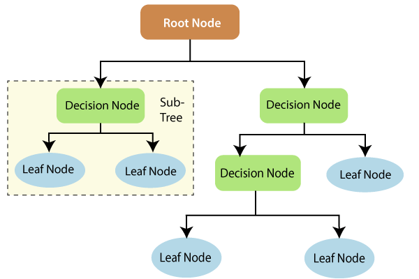
Decision tree
- They are relatively fast to construct and they produce interpretable models (if the trees are small).
- They naturally incorporate mixtures of numeric and categorical predictor variables and missing values
- They are invariant under (strictly monotone) transformations of the individual predictors. As a result, scaling and/or more general transformations are not an issue, and they are immune to the effects of predictor outliers
- They perform internal feature selection as an integral part of the procedure
- They are thereby resistant, if not completely immune, to the inclusion of many irrelevant predictor variables
- There is no need for the exclusive creation of dummy variables
- Test attributes at each node are selected on the basis of a heuristic or statistical impurity measure example, Gini, or Information Gain (Entropy).
Conditions for stopping partitioning
- All samples for a given node belong to the same class
- There are no ramaining attributes for further partitioning
- There are no samples left
Decision tree


Decision tree
Regresión

Decision tree
Clasificación

Decision tree
Criterios de separación
Entropy

Entropy
Ejemplo 1

Entropy
Ejemplo 1

Entropy
Ejemplo 1

Entropy
Ejemplo 2

Entropy
Ejemplo 2

Entropy
Ejemplo 2

Gini impurity
Gini impurity is a metric of measuring the mix of a set. The value of Gini Impurity lies between 0 and 1 and it quantifies the uncertainty at a node in a tree. So Gini Impurity tells us how mixed up or impure a set is. Now our goal with classification is to split or partition our data into as pure or unmixed sets as possible. If we reach at a 0 Gini Impurity value we stop dividing the tree further

Gini impurity

Gini impurity

Gini impurity

Ejemplo

Ejemplo

Ejemplo

Ejemplo

Ejemplo

Decision tree hyperparametrs

Ensemble learning
The goal of ensemble methods is to combine the predictions of several base estimators built with a given learning algorithm in order to improve generalizability / robustness over a single estimator. By combining individual models, the ensemble model tends to be more flexible (less bias) and less data-sensitive (less variance).
- Bagging it is to build several estimators independently in a parallel way and then to average their predictions. the combined estimator is usually better than any of the single base estimator because its variance is reduced.
- Boosting: base estimators are built sequentially and one tries to reduce the bias of the combined estimator. Each individual model learns from mistakes made by the previous model.
Bagging vs Boosting

Bagging vs Boosting

Bagging vs Boosting

Bagging vs Boosting

Bagging
Base models that are often considered for bagging are models with high variance but low bias

Bagging

Bagging

Bagging

Bagging

Bagging

Bagging

Ej- Random forest

Ej- Random forest
Random forest is an ensemble model using bagging as the ensemble method and decision tree as the individual model.

Ej- Random forest
Se puede realiza en términos de observaciones y/o en términos de predictores

Ej- Random forest

Ej- Random forest
We see that the vertical width of the red tube, formed by the Random Forests is smaller than the Decision Trees’ black tube. So, Random Forests have a lower variance than Decision Trees, as expected. Furthermore, it seems that the averages (the middle) of the two tubes are the same which means that the process of averaging did not change the bias. We still hit the underlying true function 3sin(x)+x quite well.
https://towardsdatascience.com/understanding-the-effect-of-bagging-on-variance-and-bias-visually-6131e6ff1385Ej- Random forest

Boosting
Boosting is a method of converting weak learners into strong learners (low variance but high bias) --> Shallow decision trees (stump)

AdaBoost
AdaBoost (Adaptative Boosting) is a boosting ensemble model and works especially well with the decision tree. Boosting model’s key is learning from the previous mistakes, e.g. misclassification data points. AdaBoost learns from the mistakes by increasing the weight of misclassified data points.

Ej1 - AdaBoost
As you can see, the 3 points I marked with yellow are on the wrong side. For this reason, we need to increase their weight for the 2nd iteration. But how?. In the 1st iteration, we have 7 correctly and 3 incorrectly classified points. Let’s assume we want to bring our solution into a 50/50 balance situation. Then we need to multiply the weight of incorrectly classified points with (correct/incorrect) which is (7/3 ≈ 2.33). If we increase the weight of the incorrectly classified 3 points to 2.33, our model will be 50–50%. We keep the results of 1st classification in our minds and go to the 2nd iteration.

Ej1 - AdaBoost
In the 2nd iteration, the best solution is as on the left. Correctly classified points have a weight of 11, whereas incorrectly classified points’ weight is 3. To bring the model back to a 50/50 balance, we need to multiply the incorrectly classified points’ weight by (11/3 ≈ 3.66). With new weights, we can take our model to the 3rd iteration.

Ej1 - AdaBoost
The best solution for the 3rd iteration is as on the left. The weight of the correctly classified points is 19, while the weight of the incorrectly classified points is 3 (once again). We can continue the iterations, but let’s assume that we end it here. We have now reached the stage of combining the 3 weak learners. But how do we do that?

Ej1 - AdaBoost
ln(correct/incorrect) seems to give us the coefficients we want.

Ej1 - AdaBoost
If we consider the blue region as positive and the red region as negative; we can combine the result of 3 iterations like the picture on the left.

Ej2 - AdaBoost

Ej2 - AdaBoost

Ej2 - AdaBoost

Ej2 - AdaBoost

Ej2 - AdaBoost


Deep learning


Perceptron
A perceptron is a binary classification algorithm modeled after the functioning of the human brain—it was intended to emulate the neuron. The perceptron, while it has a simple structure, has the ability to learn and solve very complex problems.

Multilayer Perceptron
A multilayer perceptron (MLP) is a group of perceptrons, organized in multiple layers, that can accurately answer complex questions. Each perceptron in the first layer (on the left) sends signals to all the perceptrons in the second layer, and so on. An MLP contains an input layer, at least one hidden layer, and an output layer.


Deep learning

Adaline

Deep learning

Deep learning

Deep learning

Deep learning

Deep learning

Deep learning

Deep learning

Deep learning

Deep learning

Deep learning

Función de activación

Universal Approximation Theorem
A feedforward network with a single layer is sufficient to represent any function, but the layer may be infeasibly large and may fail to learn and generalize correctly. — Ian Goodfellow.

Universal Approximation Theorem

Universal Approximation Theorem

Función de activación

Función de activación

Función de activación

Función de activación

Función de activación

Función de activación

Función de activación

Función de activación
which one to prefer?
- As a rule of thumb, you can start with ReLu as a general approximator and switch to other functions if ReLu doesn't provide better results.
- For CNN, ReLu is treated as a standard activation function but if it suffers from dead neurons then switch to LeakyReLu
- Always remember ReLu should be only used in hidden layers
- For classification, Sigmoid functions(Logistic, tanh, Softmax) and their combinations work well. But at the same time, it may suffer from vanishing gradient problem
- For RNN, the tanh activation function is preferred as a standard activation function.
Backpropagation

Backpropagation

Hyperparameters

Hyperparameters


Redes Neuronales Convolucionales
ConvNets -CNN-

ConvNets -CNN-


The Kernel
The objective of the Convolution Operation is to extract the high-level features such as edges, from the input image.

The Kernel

The Kernel

The Kernel

Stride

Stride & Padding
We can observe that the size of output is smaller that input. To maintain the dimension of output as in input , we use padding. Padding is a process of adding zeros to the input matrix symmetrically. In the following example,the extra grey blocks denote the padding. It is used to make the dimension of output same as input.

Stride & Padding


Types of pooling
There are two types of Pooling: Max Pooling and Average Pooling. Max Pooling returns the maximum value from the portion of the image covered by the Kernel. On the other hand, Average Pooling returns the average of all the values from the portion of the image covered by the Kernel.


Flattering
Now that we have converted our input image into a suitable form for our Multi-Level Perceptron, we shall flatten the image into a column vector. The flattened output is fed to a feed-forward neural network and backpropagation applied to every iteration of training. Over a series of epochs, the model is able to distinguish between dominating and certain low-level features in images and classify them using the Softmax Classification technique.

Fully connected layer
Adding a Fully-Connected layer is a (usually) cheap way of learning non-linear combinations of the high-level features as represented by the output of the convolutional layer. The Fully-Connected layer is learning a possibly non-linear function in that space.

CNN

CNN

CNN

Ejemplo 3D
CNN
Redes Neuronales Recurrentes


RNN

RNN

RNN

RNN

RNN

RNN


Many to one
RNN

RNN


RNN

Long Short Term memory (LSTM)

Long Short Term memory (LSTM)

Long Short Term memory (LSTM)

Generalized Linear Models (GLM's)
General Linear Models
$ Y_i=\beta_0+\beta_1x_1+\beta_2x_2+...+\beta_nx_n+\epsilon $ $ Y_i \sim N(u,\sigma^2) $- Our response variable and error term follows Normal distribution.
- Relationship between response and explanatory variable is linear.
- Errors are homoscedastic and non-correlated.
- If the independent explanatory variables are not correlated.
Generalized Linear Models (GLMs)
The generalized linear model (GLM) is a flexible generalization of General Linear model that allows for response variable that have error distribution models normal and non-normal distribution as well. It allows the linear predictor (e.g. $b_0+b_1*X$)to be related to the response via a function which is called link function.
- Random Component:-means the probability distribution of response yi.
- Systematic Component:- linear combination of explanatory variables.
- Link Function:- defines how the expected value of response is related to the linear predictor of explanatory variables.
Note: General Linear Models are specific GLMS when errors are independent and follows normal distribution. And the link function is identity because we model the mean directly in case of General Linear Models.
Modelo Lineal
$ y=\beta_0+\beta_1x_1+\beta_2x_2+...+\beta_nx_n+\epsilon $GAMs
$ G(y)=\beta_0+W_1F_1x_1+W_2F_2x_2+...+W_nF_nx_n+\epsilon $Donde:
F1(X1), F1(X2), …. Fn(Xn) are non-parametric functions (smoothing functions)
G(Y) is a link function connecting the expected value to input features X1,X2….Xn
Supuestos de GML
- The data are independently distributed, i.e., cases are independent.
- The dependent variable does NOT need to be normally distributed, but it typically assumes a distribution from an exponential family (e.g. binomial, Poisson, multinomial, normal, etc.).
- A GLM does NOT assume a linear relationship between the response variable and the explanatory variables, but it does assume a linear relationship between the transformed expected response in terms of the link function and the explanatory variables; e.g., for binary logistic regression
- Explanatory variables can be nonlinear transformations of some original variables.
- The homogeneity of variance does NOT need to be satisfied. In fact, it is not even possible in many cases given the model structure.
- Errors need to be independent but NOT normally distributed.
- Parameter estimation uses maximum likelihood estimation (MLE) rather than ordinary least squares (OLS).
Hierarchical Linear Models (HLM)

Random Intercept model

Random slope model

Random slope model

Covariance
