ANÁLISIS GEOESPACIAL
Prof. Edier Aristizábal

First Law of Geography
“Everything is related to everything else, but near things are more related than distant things."
Waldo R. Tobler (1970)
Second Law of Geography
“Geographic variables exhibit uncontrolled variance."
Goodchild (2004)
Introducción
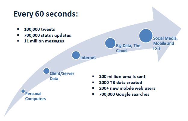
La era de los datos
Almacenamiento de datos

Almacenamiento de datos
Los kilobytes eran almacenados en discos, megabytes fueron almacenados en discos duros, terabytes fueron almacenados en arreglos de discos, y petabytes son almacenados en la nube.

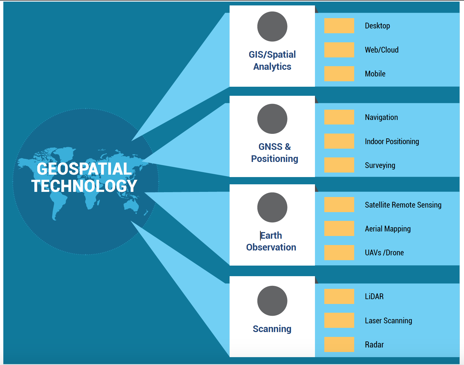
¿Por qué lo espacial es especial?

¿Por qué lo espacial es especial?

¿Por qué lo espacial es especial?
Charles Picquet (1832)

Dr. John Snow (1854)

Fotografía aérea (1858)
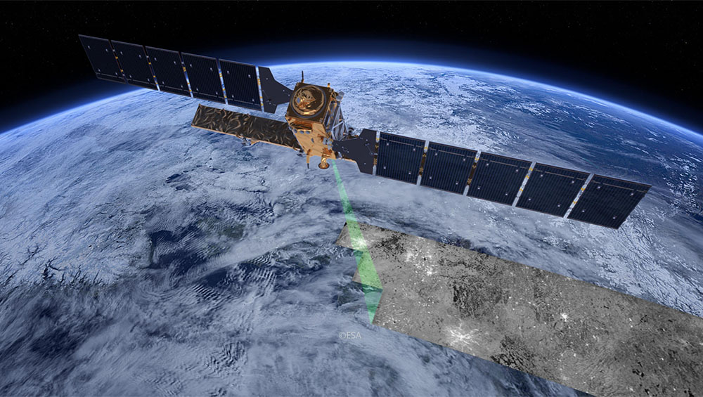
Sensores remotos (1972)
Roger F. Tomlinson (1960)

Actualidad

Actualidad

Actualidad
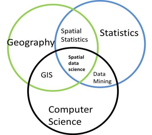
Ciencia de Datos Geoespaciales
La ciencia de datos geoespaciales (GDS) es un subconjunto de la Ciencia de Datos que se enfoca en las características únicas de los datos espaciales, yendo más allá de simplemente observar dónde ocurren las cosas para entender por qué ocurren allí
La extracción de información significativa a partir de datos que involucran ubicación, proximidad geográfica y/o interacción espacial mediante el uso de técnicas específicamente diseñadas para tratar adecuadamente los datos espaciales.
La ciencia de datos espaciales es un campo interdisciplinario que se enfoca en analizar e interpretar datos que tienen un componente geográfico o espacial. La ciencia de datos espaciales trabaja con datos vinculados a una ubicación específica en la superficie de la Tierra.
Análisis espacial
- Manipulación de datos espaciales mediante sistemas de información geográfica (SIG),
- Análisis de datos espaciales de forma descriptiva y exploratoria (Python, JS, R...),
- Estadística espacial que emplea procedimientos estadísticos para investigar si se pueden hacer inferencias
- Modelado espacial que implica la construcción de modelos para identificar relaciones y predecir resultados en un contexto espacial.
Análisis espacial
La ciencia de datos espaciales fusiona varias áreas, incluyendo:
- Análisis Geoespacial: El estudio e interpretación de datos geográficos mediante algoritmos espaciales.
- Aprendizaje Automático: El uso de modelos estadísticos y algoritmos de aprendizaje automático para hacer predicciones o descubrir patrones en datos geoespaciales.
- Visualización de Datos: Creación de mapas, gráficos y otras visualizaciones que representan la distribución espacial de los datos.
- Estadística Espacial: Aplicación de técnicas estadísticas para entender patrones y relaciones espaciales.
Análisis espacial

Herramientas
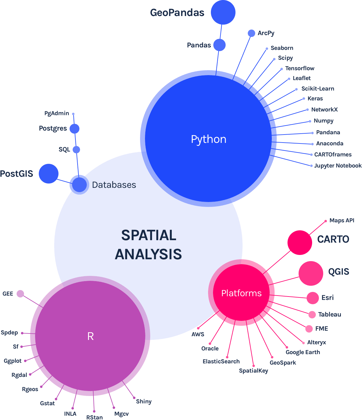
https://carto.com/what-is-spatial-data-science/
Ambiente de trabajo
Índice TIOBE - Popularidad de lenguajes de programación

Python
Python es rápido para desarrollar: Como el código no necesita ser compilado y construido, el código Python puede ser modificado y ejecutado fácilmente. Esto permite un ciclo de desarrollo rápido.
Python no es tan rápido en ejecución: El código Python es un poco más lento en comparación con lenguajes convencionales como C, C++, etc.
Python es interpretado: Python no necesita compilación a código binario, lo que hace que Python sea más fácil de usar y mucho más portable que otros lenguajes de programación.
Python es orientado a objetos: Muchos lenguajes de programación modernos soportan programación orientada a objetos. ArcGIS y QGIS están diseñados para trabajar con lenguajes orientados a objetos, y Python cumple con este requisito.
Paquetes

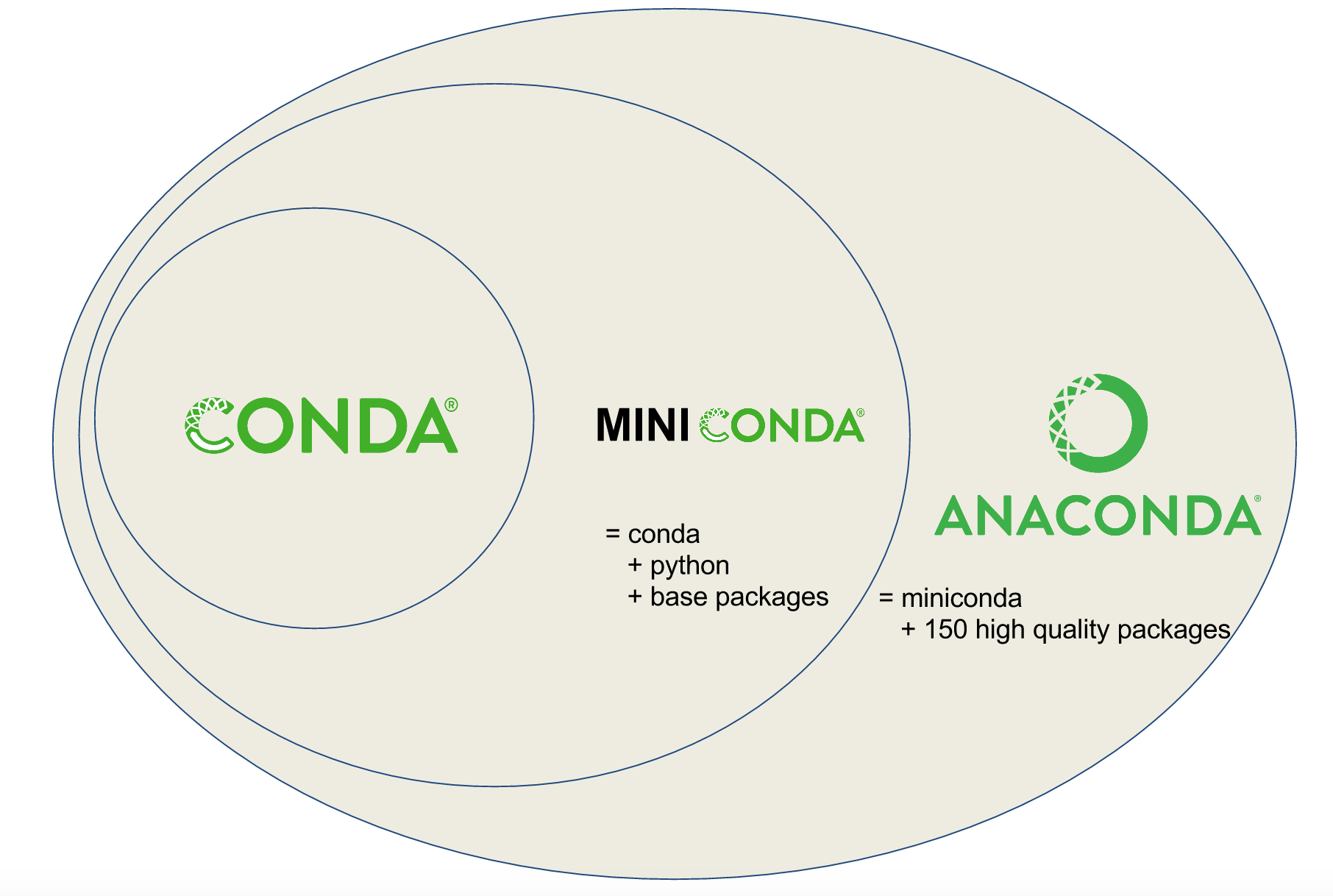
Conda

PIP

Docker

R

RStudio

Javascript

Google Earth Engine

Material de apoyo
Distribución de datos

Distribución de frecuencia e histogramas
La tabla de distribución de frecuencia es una tabla que almacena las categorías (también llamadas "bins"), la frecuencia, la frecuencia relativa y la frecuencia relativa acumulada de una variable continua de intervalo único
La frecuencia de una categoría o valor particular (también llamado "observación") de una variable es el número de veces que la categoría o el valor aparece en el conjunto de datos.
La frecuencia relativa es la proporción (%) de las observaciones que pertenecen a una categoría. Se utiliza para entender cómo se distribuye una muestra o población entre los bins (se calcula como frecuencia relativa = frecuencia/n)
La frecuencia relativa acumulada de cada fila es la suma de la frecuencia relativa de esa fila y las anteriores. Nos indica qué porcentaje de una población (observaciones) se acumula hasta ese bin. La última fila debe ser 100%.
Un histograma de densidad de probabilidad se define de manera que (i) El área de cada barra es igual a la frecuencia relativa (probabilidad) del bin correspondiente, (ii) El área total del histograma es igual a 1
Distribución de frecuencia
Histogramas & bins
Distribución de frecuencia

Distribución de frecuencia

Teorema del Límite Central
Cuando recolectamos muestras suficientemente grandes de una población, las medias de las muestras tendrán una distribución normal. Incluso si la población no tiene distribución normal.
Diagrama de caja (Box plot)
Un diagrama de caja es una representación gráfica de las estadísticas descriptivas clave de una distribución.
Las características de un diagrama de caja son
- La caja se define usando el cuartil inferior Q1 (25%; borde vertical izquierdo de la caja) y el cuartil superior Q3 (75%; borde vertical derecho de la caja). La longitud de la caja es igual al rango intercuartílico IQR = Q3 - Q1.
- La mediana se representa mediante una línea dentro de la caja. Si la mediana no está centrada, existe asimetría.
- Para rastrear y representar valores atípicos, debemos calcular los bigotes, que son las líneas que parten de los bordes de la caja y se extienden hasta el último objeto no considerado atípico.
- Los objetos que se encuentran más allá de 1.5 IQR se consideran valores atípicos.
- Los objetos que se encuentran a más de 3.0 IQR se consideran valores atípicos extremos, y aquellos entre (1.5 IQR y 3.0 IQR) se consideran valores atípicos leves. Se puede cambiar el coeficiente 1.5 o 3.0 a otro valor según las necesidades del estudio, pero la mayoría de los programas estadísticos usan estos valores por defecto.
- Los bigotes no necesariamente se extienden hasta 1.5 IQR sino hasta el último objeto que se encuentra antes de esta distancia desde los cuartiles superior o inferior.
Diagrama de caja

Diagrama de caja

Diagrama de caja

Gráfico QQ
El gráfico QQ normal es una técnica gráfica que grafica los datos contra una distribución normal teórica que forma una línea recta
Un gráfico QQ normal se utiliza para identificar si los datos tienen distribución normal
Si los puntos de datos se desvían de la línea recta y aparecen curvas (especialmente al inicio o al final de la línea), se viola el supuesto de normalidad.
QQ Plot

Diagrama de dispersión
Un diagrama de dispersión muestra los valores de dos variables como un conjunto de coordenadas de puntos
Un diagrama de dispersión se utiliza para identificar las relaciones entre dos variables y rastrear posibles valores atípicos.
Inspeccionar un diagrama de dispersión permite identificar asociaciones lineales u otros tipos de asociaciones
Si los puntos tienden a formar un patrón lineal, una relación lineal entre las variables es evidente. Si los puntos están dispersos, la correlación lineal es cercana a cero y no se observa asociación entre las dos variables. Los puntos que se encuentran más alejados en la dirección x o y (o ambas) son posibles valores atípicos
Visualización D3js: 4 variables
Distribuciones de probabilidad estadística
Una distribución estadística describe cómo se distribuyen o dispersan los valores de una variable. Nos indica la probabilidad de diferentes resultados

Distribuciones de probabilidad estadística
Distribuciones de probabilidad estadística

Distribución subyacente de los datos

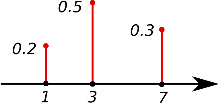
PMF: Función de Masa de Probabilidad
Devuelve la probabilidad de que una variable aleatoria discreta X sea igual a un valor de x. La suma de todos los valores es igual a 1. La PMF solo se puede usar con variables discretas.
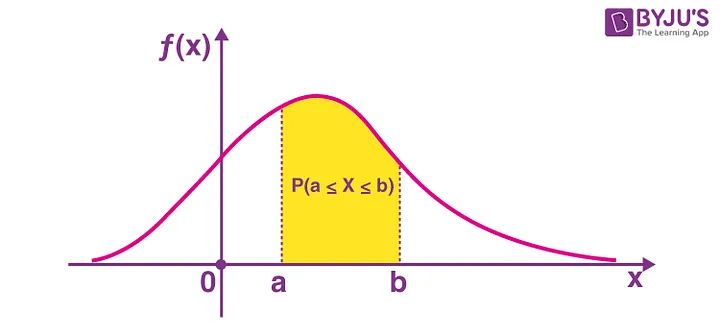
PDF: Función de Densidad de Probabilidad
Es como la versión de la PMF para variables continuas. Devuelve la probabilidad de que una variable aleatoria continua X esté en un rango determinado.
CDF: Función de Distribución Acumulada
Devuelve la probabilidad de que una variable aleatoria X tome valores menores o iguales a x.

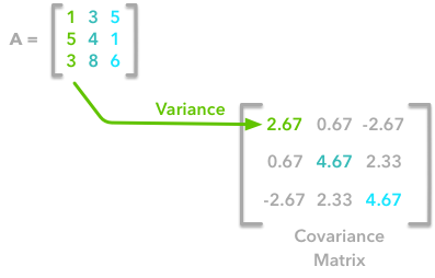
Matriz de covarianza
La covarianza es una medida del grado en que dos variables varían juntas (es decir, cambian en la misma dirección lineal). La covarianza Cov(X, Y) se calcula como:
$cov_{x,y}=\frac{\sum_{i=1}^{n}(x_{i}-\bar{x})(y_{i}-\bar{y})}{n-1}$donde $x_i$ es el valor de la variable X del i-ésimo objeto, $y_i$ es el valor de la variable Y del i-ésimo objeto, $\bar{x}$ es el valor medio de la variable X, $\bar{y}$ es el valor medio de la variable Y.
Para covarianza positiva, si la variable X aumenta, entonces la variable Y también aumenta. Si la covarianza es negativa, las variables cambian de manera opuesta (una aumenta, la otra disminuye). Una covarianza cero indica que no hay correlación entre las variables.
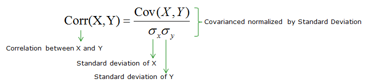
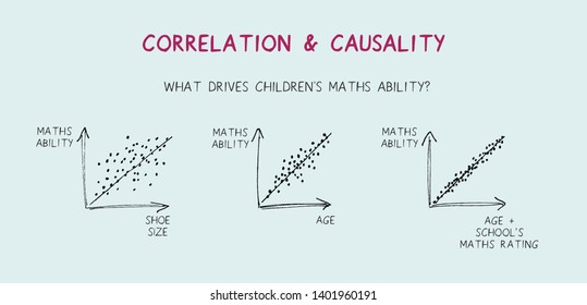
Coeficiente de correlación
El coeficiente de correlación $r_{(x, y)}$ analiza cómo dos variables (X, Y) están relacionadas linealmente. Entre las métricas de coeficiente de correlación disponibles, la más utilizada es el coeficiente de correlación de Pearson (también llamado correlación producto-momento de Pearson),
$r_{(x, y)} = \frac{\text{cov}(X,Y)}{s_x s_y}$La correlación es una medida de asociación y no de causalidad.

Pensamiento espacial
Fenómenos espaciales
La suposición estadística de independencia e idéntica distribución (iid) es equivalente a asumir datos homogéneos. En otras palabras, la media y la varianza de una variable aleatoria son constantes entre las observaciones, al igual que todos los demás momentos (asimetría y curtosis).
La pregunta a abordar es sí la media y la varianza de algún fenómeno varían o no entre las regiones en las que se divide un paisaje?
Dependencia espacial
La dependencia espacial implica que las observaciones en una región están correlacionadas con las de las regiones vecinas (Fletcher, 2018). La dependencia espacial se mide frecuentemente mediante la covarianza y, por lo tanto, es una propiedad de segundo orden - covarianza.
Heterogeneidad espacial
la heterogeneidad espacial se refiere a los efectos del espacio sobre las unidades muestrales, en las cuales la media varía de un lugar a otro (Zhang, 2023). Por lo tanto, la heterogeneidad espacial es una propiedad de primer orden - la media (Wang, 2022)
Tipos de análisis espaciales
- Análisis de patrones de puntos: modelado de eventos en un dominio (D) aleatorio. En el análisis de patrones de puntos, el enfoque es diferente porque aquí se trata de estudiar la distribución de eventos puntuales en el espacio, y dichos puntos (que representan eventos u ocurrencias) son considerados como realizaciones de un proceso estocástico.
- Análisis de datos areales o discretos (lattice): modelado donde el dominio (D) de los datos espaciales es discreto y fijo, donde las regiones espaciales que definen el dominio pueden tener formas regulares (grid o píxeles) o formas irregulares (polígonos).
- Análisis geoestadístico: modelado donde el dominio (D) de los datos espaciales es una superficie continua (campos) y fija. En geoestadística como en análisis de datos discretos, el atributo no es lo que define si los datos son espacialmente continuos o discretos; en este caso la continuidad proviene del hecho de que el dominio (D) permite realizar mediciones en cualquier lugar.
Escala
La escala también es importante porque puede informar sobre el muestreo para la experiencia de entrenamiento. El aprendizaje es más confiable cuando la distribución de las muestras en la experiencia de entrenamiento es similar a la distribución de la experiencia de prueba. En muchos estudios geográficos, el entrenamiento se realiza con datos de un área geográfica específica. Esto hace que sea difícil usar el modelo entrenado para otras regiones geográficas porque la distribución de los conjuntos de datos de prueba y entrenamiento no es similar, debido a la heterogeneidad espacial.
Esto significa que la estrategia de muestreo para el conjunto de datos de entrenamiento es esencial para cubrir la heterogeneidad del fenómeno de interés en el marco espacial de estudio. Al aumentar la extensión del área de estudio, más procesos y factores ambientales contextuales pueden alterar la variable y resultar en no estacionariedad al entrelazar patrones espaciales de diferentes escalas o efectos inconsistentes de los procesos en diferentes regiones.
Efectos de primer y segundo orden
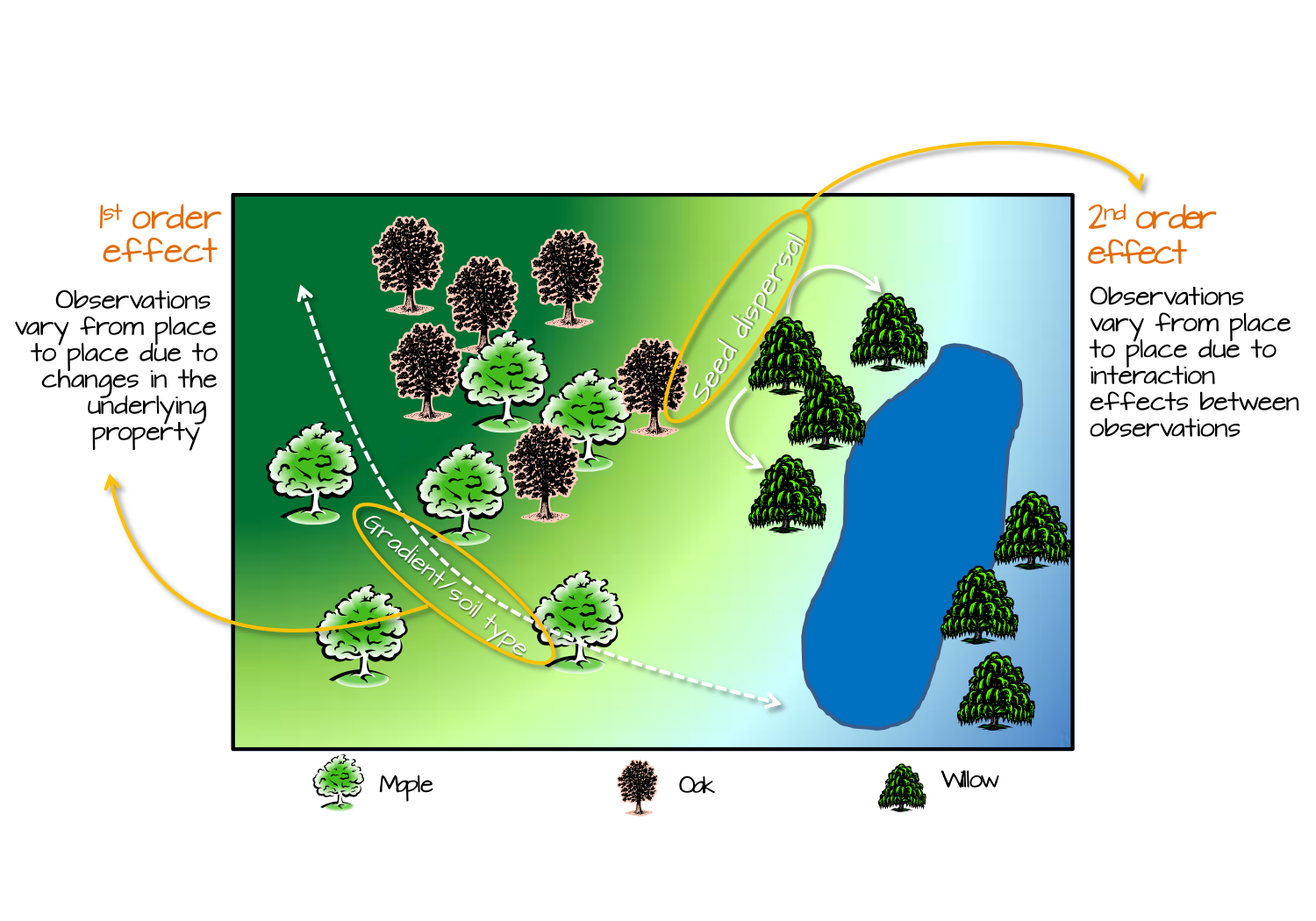
La distribución de densidad de árboles puede estar influenciada por efectos de 1er orden como el gradiente de elevación o la distribución espacial de las características del suelo; y por efectos de 2do orden como los procesos de dispersión de semillas donde el proceso es independiente de la ubicación y, en cambio, dependiente de la presencia de otros árboles.
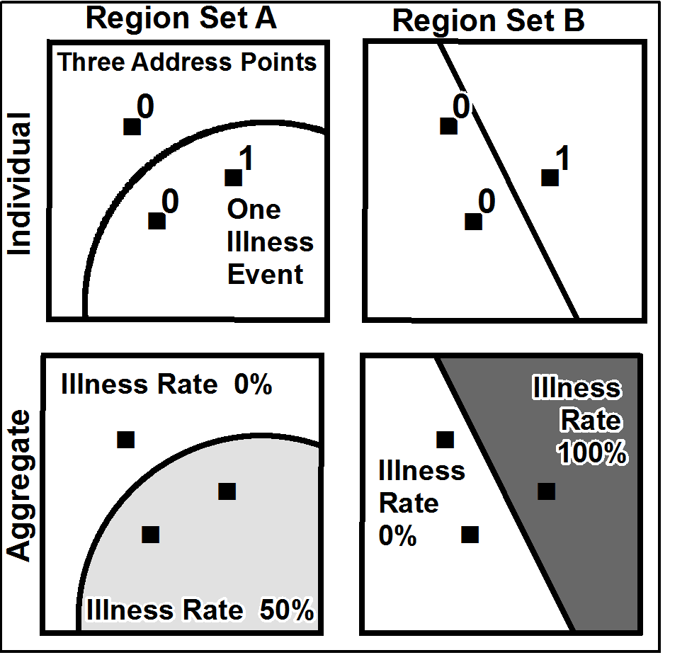
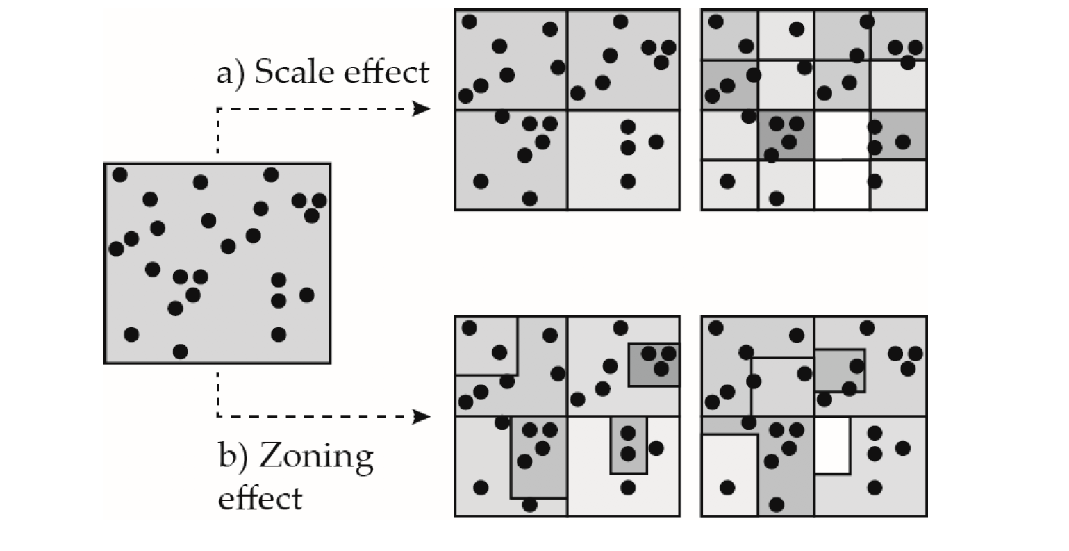
MAUP
El problema de la Unidad de Área Modificable (MAUP) se refiere a la influencia que el diseño de las zonas tiene sobre los resultados del análisis. Una designación diferente probablemente llevaría a resultados diferentes.
MAUP
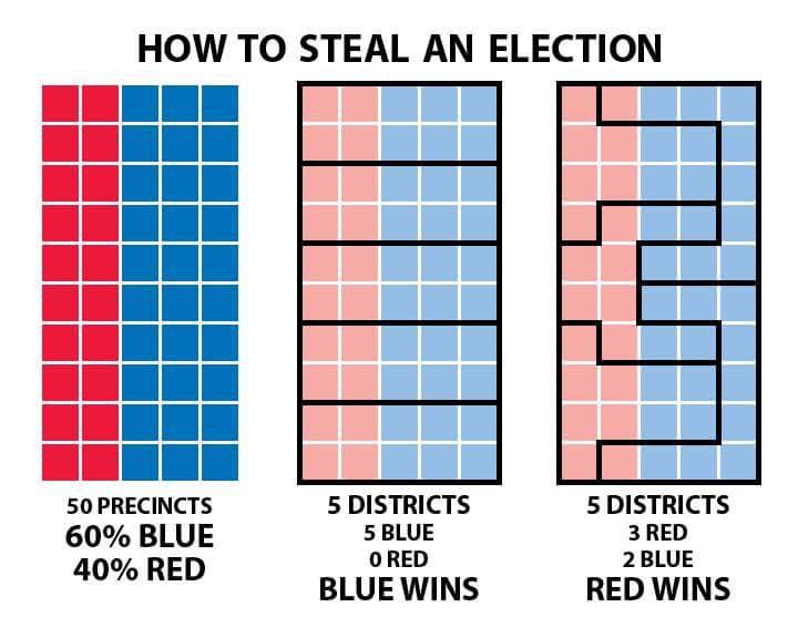
MAUP
Existen dos tipos de sesgos en el MAUP:
Efecto zonal
El efecto zonal ocurre cuando se agrupan datos por varios límites artificiales. En este tipo de error MAUP, cada límite subsiguiente produce diferencias analíticas importantes.
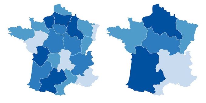
Efecto de escala
El efecto de escala ocurre cuando los mapas muestran diferentes resultados analíticos a diferentes niveles de agregación. A pesar de usar los mismos puntos, cada unidad sucesivamente más pequeña cambia el patrón.


Efecto de borde

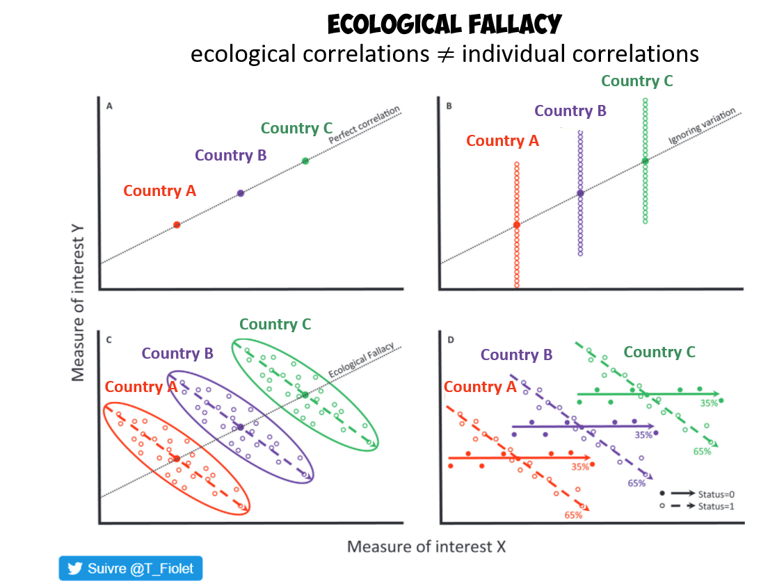
Falacia ecológica
Este problema ocurre cuando una relación que es estadísticamente significativa a un nivel de análisis se asume que también es válida a un nivel más detallado. Este es un error típico que ocurre cuando usamos datos agregados para describir el comportamiento de individuos.

Efecto de vecindario
Las características de las propiedades vecinas pueden tener cierto impacto sobre la misma característica en los vecinos.
Los efectos locales se refieren a patrones o relaciones espaciales que varían a nivel de una unidad espacial específica o en un vecindario pequeño.
Los efectos globales son los efectos que se suponen constantes a lo largo de todo el espacio.
Efectos de X sobre y
Los efectos directos son los efectos que una variable independiente tiene sobre la variable dependiente en la misma unidad espacial.
Los efectos indirectos son los efectos que una variable explicativa en una unidad tiene sobre la variable dependiente en otras unidades vecinas.
El término spillover es sinónimo de efectos indirectos, pero a veces se usa de forma más cualitativa para describir el fenómeno general de propagación del efecto entre unidades
Los efectos marginales son la derivada de la variable dependiente respecto a una variable explicativa.
Los efectos fijos (fixef effects) capturan características específicas y constantes de cada unidad. Se modelan como parámetros específicos para cada unidad.
Los efectos aleatorios (random effects) se usan en modelos jerarquicos para entender el patron general, se estiman como una varianza común que describe la variabilidad entre las unidades.
Efectos de X sobre y
| Tipo de efecto | ¿Qué representa? | ¿Depende de la estructura espacial? | ¿Unidad específica? |
|---|---|---|---|
| Directo | Efecto de X sobre Y en la misma unidad | ✅ | ✅ |
| Indirecto | Efecto de X sobre Y en unidades vecinas | ✅ | ❌ |
| Spillover | Propagación espacial de los efectos | ✅ | ❌ |
| Marginal | Cambio en Y ante un cambio unitario en X | ✅ (en modelos espaciales) | Depende |
| Fijo | Diferencias no observadas por unidad | ❌ (no espacial por defecto) | ✅ |
| Aleatorio | Variabilidad aleatoria entre unidades | ✅ (Modelos Jerárquicos) | ❌ |
Datos espaciales
Datos

Datos espaciales
Los datos espaciales son datos geográficamente referenciados, dados en ubicaciones conocidas y a menudo representados visualmente a través de mapas. Esa referencia geográfica, o el componente de ubicación de los datos, puede representarse usando cualquier número de sistemas de referencia de coordenadas, por ejemplo, longitud y latitud.
Datos geoespaciales
Los datos geoespaciales son datos sobre objetos, eventos o fenómenos que tienen una ubicación en la superficie de la tierra, incluyendo información de ubicación, información de atributos (las características del objeto, evento o fenómeno en cuestión), y a menudo también información temporal (el tiempo o periodo de vida en el que existen la ubicación y los atributos)
Los modelos son simplificaciones de la realidad

Modelos de datos espaciales
- Datos se pueden definir como hechos verificables sobre el mundo real.
- Información son datos organizados para revelar patrones y facilitar la búsqueda.
- Modelo de datos: una abstracción del mundo real que incorpora solo aquellas propiedades consideradas relevantes para la aplicación
- Estructura de datos: una representación del modelo de datos
- Formato de archivo: la representación de los datos en el hardware de almacenamiento
Los datos del mundo real deben describirse en términos de un modelo de datos, luego se debe elegir una estructura de datos para representar el modelo de datos, y finalmente se debe seleccionar un formato de archivo adecuado para esa estructura de datos.
Tipos de modelos espaciales
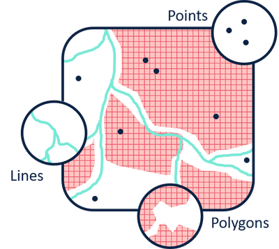
- Modelo basado en objetos (vectorial): En la vista de objetos, consideramos el mundo como una serie de entidades ubicadas en el espacio. Las entidades son (generalmente) reales. Un objeto es una representación digital de toda o parte de una entidad, que puede describirse en detalle según sus líneas límite y otros objetos que las constituyen o están relacionados con ellas.
- Modelo de campo: En la vista de campo, el mundo consiste en propiedades que varían continuamente a través del espacio. Representa datos que se consideran en cambio continuo en el espacio bidimensional o tridimensional. En un campo, cada ubicación tiene un valor (incluyendo ''no aquí'' o cero) y los conjuntos de valores tomados juntos definen el campo.
Estructura de datos
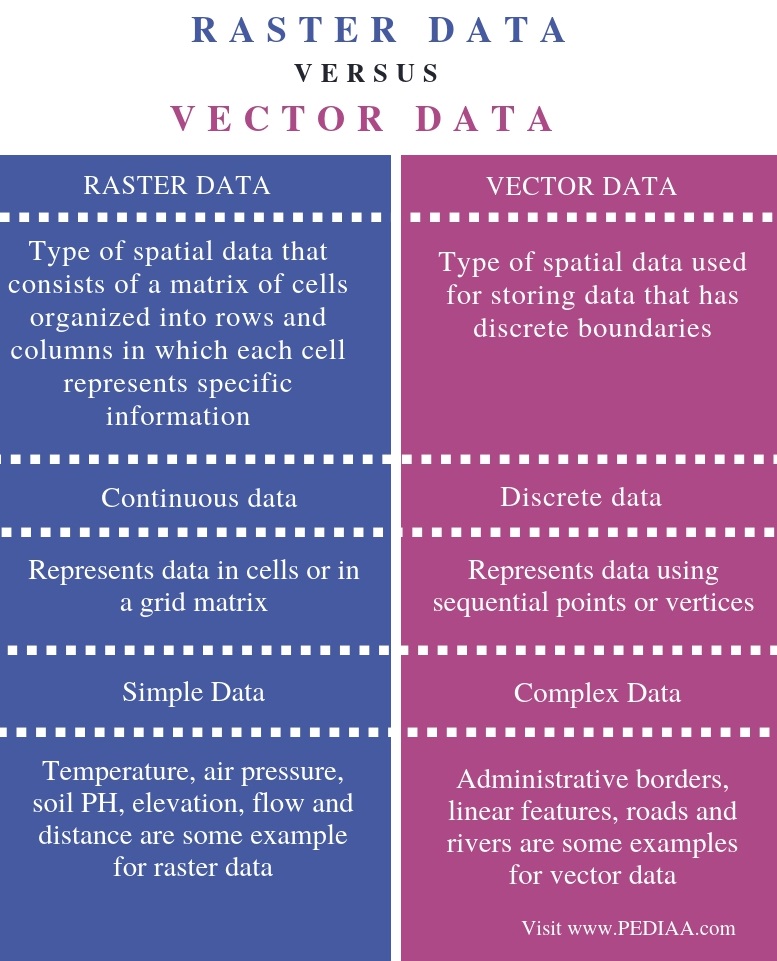
Modelo basado en objetos
Vector
Los objetos frecuentemente no son tan simples como esta visión geométrica lleva a suponer. Pueden existir en tres dimensiones espaciales, moverse y cambiar con el tiempo, tener una representación fuertemente dependiente de la escala, relacionarse con entidades que son difusas y/o tienen límites indeterminados, o incluso ser fractales.
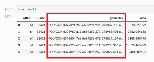
Vector (tabla geográfica)
Shapefile
Un shapefile es un formato de datos basado en archivos nativo del software ArcView. Conceptualmente, un shapefile es una clase de entidades–almacena una colección de entidades que tienen el mismo tipo de geometría (punto, línea o polígono), los mismos atributos y una extensión espacial común. A pesar de lo que su nombre pueda implicar, un shapefile "individual" está compuesto por al menos tres archivos, y hasta ocho. Cada archivo que compone un "shapefile" tiene un nombre de archivo común pero diferente tipo de extensión.
Arc-Info Interchange (e00)
Un archivo de intercambio ArcInfo, también conocido como tipo de archivo de exportación, este formato se utiliza para permitir la transferencia de una cobertura, grid o TIN, y una tabla INFO asociada entre diferentes máquinas. Este archivo tiene la extensión .e00.
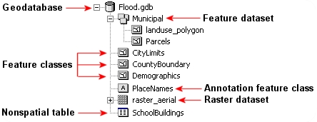
File Geodatabase
Una file geodatabase es un formato de almacenamiento de base de datos relacional. Es una estructura de datos mucho más compleja que el shapefile y consiste en una carpeta .gdb que alberga docenas de archivos. Su complejidad la hace más versátil, permitiéndole almacenar múltiples clases de entidades y habilitando definiciones topológicas. Un ejemplo del contenido de una geodatabase se muestra en la siguiente figura.
GeoPackage
Este es un formato de datos relativamente nuevo que sigue estándares de formato abierto (es decir, no es propietario). Está construido sobre SQLite (una base de datos relacional autocontenida). Su gran ventaja sobre muchos otros formatos vectoriales es su compacidad–valores de coordenadas, metadatos, tabla de atributos, información de proyección, etc., están todos almacenados en un solo archivo lo que facilita la portabilidad. Su nombre de archivo generalmente termina en .gpkg. Aplicaciones como QGIS (2.12 en adelante), R y ArcGIS reconocen este formato (ArcGIS versión 10.2.2 y superior leerá el archivo desde ArcCatalog pero requiere un script para crear un GeoPackage).
Geojson
GeoJSON es un formato de estándar abierto diseñado para representar entidades geográficas simples, junto con sus atributos no espaciales
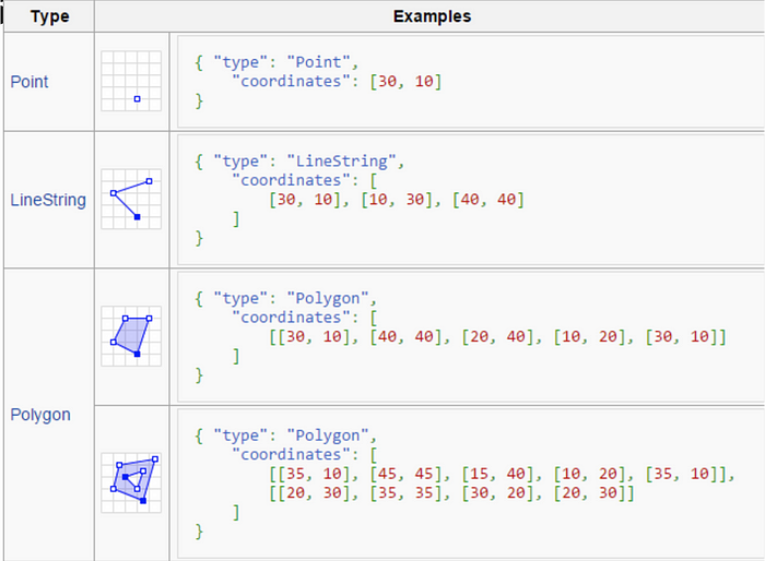
Geojson -- Geometría multiparte
Los tipos de geometría multiparte son similares a sus contrapartes de una sola parte. La única diferencia es que se agrega un nivel jerárquico más al arreglo de coordenadas, para especificar múltiples formas.

Geojson -- Colecciones de geometría
Una colección de geometría es un conjunto de varias geometrías, donde cada geometría es uno de los seis tipos listados anteriormente, es decir, cualquier tipo de geometría excepto "GeometryCollection". Por ejemplo, una "GeometryCollection" que consiste en dos geometrías, un "Point" y un "MultiLineString", se puede definir de la siguiente manera:

Geojson -- Feature (Entidad)
Un "Feature" se forma cuando una geometría se combina con atributos no espaciales, para formar un solo objeto. Los atributos no espaciales están contenidos en una propiedad llamada "properties", que contiene uno o más pares nombre-valor, uno para cada atributo. Por ejemplo, el siguiente "Feature" representa una geometría con dos atributos, llamados "color" y "area":

Geojson -- Colección de Features
Un "FeatureCollection" es, como su nombre sugiere, una colección de objetos "Feature". Los features individuales están contenidos en un arreglo que comprende la propiedad "features". Por ejemplo, un "FeatureCollection" compuesto por cuatro features se puede especificar de la siguiente manera:

http://geojson.io/
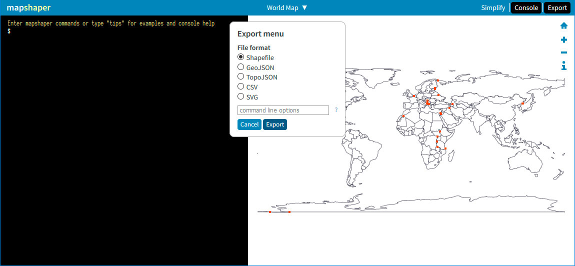
Mapshaper
Keyhole Markup Language (KML)
Formato de archivo basado en XML, utilizado para visualizar datos espaciales e información de modelado como líneas, formas, imágenes 3D y puntos en Google Earth.
Geography Markup Language (GML)
Se utiliza en el Open GIS Consortium para almacenar datos geográficos en un formato estándar de intercambio. Está basado en XML.
SVG (Scalable Vector Graphics)
Es un formato de imagen vectorial basado en XML para gráficos bidimensionales. Cualquier programa que reconozca XML puede mostrar la imagen SVG.
DWG
DWG es un formato interno de AutoCAD. Un archivo DWG es una base de datos de dibujos 2D o 3D.
Tidy data

Dataframe
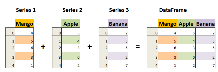
Dataframe

Modelo basado en campo
En la vista de campo, el mundo consiste en propiedades que varían continuamente a través del espacio
Raster
Formato de archivo ráster SIG
txt / ASCII (American Standard Code for Information Interchange)
Documento de texto estándar que contiene texto plano. Puede abrirse y editarse en cualquier editor de texto o procesador de palabras
Imagine
Formato de archivo Imagine de ERDAS. Consiste en un solo archivo .img. A veces va acompañado de un archivo .xml que generalmente almacena información de metadatos sobre la capa ráster.
GeoTiff
Un GeoTIFF es un archivo TIF que termina con la extensión de tres letras .tif igual que otros archivos TIF, pero un GeoTIFF contiene etiquetas adicionales que proporcionan información de proyección para esa imagen según lo especificado por el estándar GeoTIFF
Formato de archivo ráster SIG
Enhanced Compression Wavelet (ECW)
Enhanced Compressed Wavelet (de ERDAS). Un formato comprimido wavelet, a menudo con pérdida
Network Common Data Form (NetCDF)
Formato de archivo netCDF con las convenciones de metadatos Climate and Forecast (CF) para datos de ciencias de la tierra. Permite el acceso web directo a subconjuntos/agregaciones de mapas a través del protocolo OPeNDAP.
HDF5
es un formato de archivo de código abierto que soporta datos grandes, complejos y heterogéneos. HDF5 utiliza una estructura similar a un "directorio de archivos" que permite organizar los datos dentro del archivo de muchas formas estructuradas diferentes, como se podría hacer con archivos en la computadora
Mapas web
Mapas web
Un mapa web es una visualización interactiva de información geográfica, en forma de página web, que se puede usar para contar historias y responder preguntas. Los mapas web son interactivos. El término interactivo implica que el usuario puede interactuar con el mapa. Esto puede significar seleccionar diferentes capas de datos o entidades del mapa para visualizar, acercar una parte particular del mapa que le interese, inspeccionar propiedades de entidades, editar contenido existente o enviar nuevo contenido, etc.
Los mapas web son útiles para diversos propósitos, como visualización de datos en periodismo (y en otros campos), mostrando datos espaciales en tiempo real, alimentando consultas espaciales en catálogos y herramientas de búsqueda en línea, proporcionando herramientas computacionales, generando informes y mapeo colaborativo.


Herramientas

Arquitectura

Geoservidor
Web Map Service (WMS)
WMS entrega imágenes de mapas renderizadas (como PNG, JPEG) basadas en datos geográficos. Esto significa que convierte nuestros datos geoespaciales en una imagen de mapa que los usuarios pueden ver, pero con la que no pueden interactuar en términos de manipulación de datos. El uso de WMS es ideal cuando el requisito principal es mostrar una representación visual de los datos geográficos sin necesidad de interactuar con sus elementos individuales.
Web Feature Service (WFS)
WFS ofrece acceso a datos vectoriales geográficos en bruto (como puntos, polilíneas, polígonos). Esto significa que los usuarios pueden interactuar, consultar e incluso modificar directamente tanto los datos espaciales como los atributos. El uso de WFS es ideal para escenarios donde los usuarios necesitan interactuar directamente con los datos geoespaciales y, posiblemente, editarlos.
Web Map Tile Service (WMTS)
Entrega teselas de mapas pre-renderizadas, generalmente en formatos como PNG o JPEG. En lugar de renderizar la vista completa del mapa en tiempo real como lo hace WMS, WMTS utiliza teselas pre-generadas para componer rápidamente una vista de mapa basada en las operaciones de zoom y desplazamiento del usuario. El uso de WMTS es más adecuado para aplicaciones que requieren una navegación y visualización de mapas rápida, donde los datos son relativamente estáticos y no necesitan actualizaciones frecuentes.
Raster tiles: las capas de teselas suelen estar compuestas de imágenes PNG. Tradicionalmente, cada imagen PNG tiene un tamaño de 256 × 256 píxeles.
Vector tiles: las teselas vectoriales se distinguen por la capacidad de rotar el mapa mientras las etiquetas mantienen su orientación horizontal, y por la capacidad de hacer zoom de manera suave—sin la estricta división en niveles de zoom discretos que tienen las capas de teselas ráster.
Capas de teselas

Capas de teselas

https://a.tile.openstreetmap.org/2/1/3.png
Nivel de zoom

Nivel de zoom

Teselas vectoriales

Ejemplo
Web Coverage Service (WCS)
WCS proporciona acceso a datos ráster geoespaciales en bruto. A diferencia de WMS, que solo devuelve imágenes de datos, WCS devuelve los datos en bruto que representan los valores reales subyacentes de un conjunto de datos ráster. El uso de WCS es ideal cuando los usuarios necesitan los valores reales de los píxeles de un conjunto de datos ráster. Esto es importante para tareas científicas, analíticas y de modelado donde los datos en bruto, en lugar de la representación visual, son esenciales.
Web Processing Service (WPS)
WPS permite la ejecución de procesos geoespaciales en el lado del servidor. Esto significa que, en lugar de solo recuperar o mostrar datos, los usuarios pueden realizar varias operaciones sobre esos datos, como análisis de buffer, intersección, unión, etc. El uso de WPS es esencial cuando se requieren cálculos geoespaciales en tiempo real, aprovechando las capacidades de procesamiento del lado del servidor.
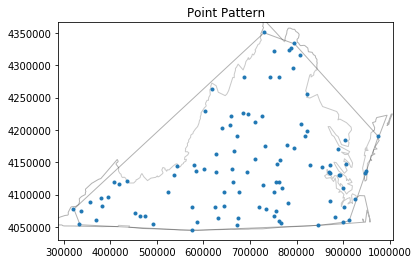
Patrón de puntos
Análisis de patrones de puntos
Análisis de patrones de puntos
Los puntos son entidades espaciales que pueden entenderse de dos maneras fundamentalmente diferentes:
- Los puntos son eventos (análisis sobre DÓNDE ocurren las cosas). Aquí, la ubicación del punto es el dato. No hay otra variable. Solo te interesa saber si hay patrones en esas ubicaciones. Un patrón de puntos consiste en un conjunto de eventos ubicados en ciertos lugares, donde cada evento representa una única instancia del fenómeno de interés.
- Los puntos son lugares donde tomaste una medida (análisis sobre QUÉ VALOR tiene algo en diferentes lugares). Una observación que ocurre en un punto también puede verse como un sitio de medición de un proceso geográficamente continuo subyacente. Este enfoque implica que tanto la ubicación como la medición importan.
Análisis de patrones de puntos
El análisis de patrones de puntos se ocupa de la visualización, descripción, caracterización estadística y modelado de patrones de puntos, tratando de comprender el proceso generador que da lugar y explica los datos observados. Las preguntas comunes en este campo incluyen:
- ¿Cómo se ve el patrón?
- ¿Cuál es la naturaleza de la distribución de los puntos?
- ¿Existe alguna estructura en la forma en que se disponen las ubicaciones en el espacio? Es decir, ¿los eventos están agrupados o están dispersos?
- ¿Por qué ocurren los eventos en esos lugares y no en otros?
Proceso & Patrón
El proceso se refiere al mecanismo subyacente que está en funcionamiento para generar el resultado que observamos. Debido a su naturaleza abstracta, no lo vemos directamente. Sin embargo, en muchos contextos, el foco principal del análisis es aprender sobre qué determina un fenómeno dado y cómo se combinan esos factores para generarlo. En este contexto, el “proceso” está asociado con el cómo.
Por otro lado, el patrón se refiere al resultado de ese proceso. En algunos casos, es la única evidencia del proceso que podemos observar y, por lo tanto, el único insumo con el que contamos para reconstruirlo. Aunque observable directamente y, quizás, más fácil de abordar, el patrón es solo un reflejo del proceso.
El verdadero desafío no es caracterizar el patrón, sino usarlo para deducir el proceso.
Proceso & Patrón
El Proceso espacial es una descripción de cómo puede generarse un patrón espacial.
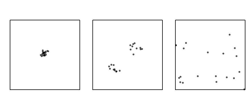
Existen tres tipos principales de proceso espacial:
- Aleatorio (CSR – Complete Spatial Randomness): Los eventos se distribuyen sin una estructura
reconocible
- Existe una probabilidad igual de ocurrencia de eventos en cualquier ubicación dentro de la región de estudio (también llamado estacionariedad de primer orden).
- La ubicación de un evento es independiente de las ubicaciones de otros eventos (también llamado estacionariedad de segundo orden).
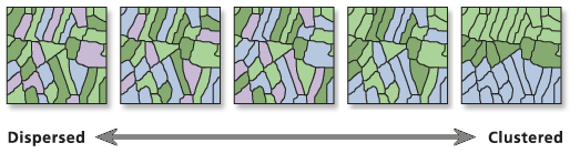
- Disperso (Regular/Uniforme): Es un proceso que hace que los eventos se dispongan lo más alejados posible entre sí; los eventos tienden a distribuirse de manera uniforme.
- Agrupado (Clustered): Los puntos tienden a aparecer juntos en grupos o “clústeres”. Puede ser resultado de un proceso subyacente.
Análisis de patrones de puntos
Existen dos métodos principales (interrelacionados) para analizar patrones de puntos: los métodos basados en la distancia y los métodos basados en la densidad.
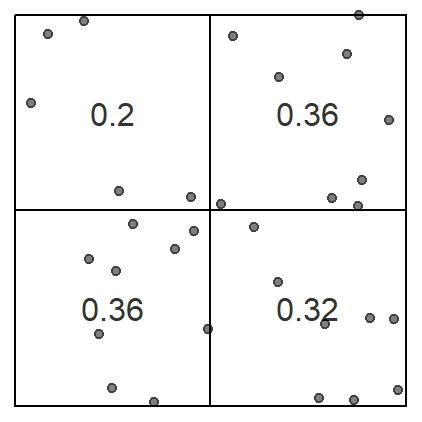
- Métodos basados en densidad --> Ubicación absoluta utilizan la intensidad de ocurrencia de eventos en el espacio. Por esta razón, describen mejor los efectos de primer orden. Los métodos de estimación por kernel son ejemplos comunes de este enfoque. En los métodos de conteo por cuadrantes, el espacio se divide en una cuadrícula regular (como una malla de cuadrados o hexágonos) de área unitaria.
- Métodos basados en distancia --> Ubicación relativa emplean las distancias entre eventos y describen los efectos de segundo orden. Estos métodos incluyen el método del vecino más cercano, las funciones de distancia G y F, la función de distancia K de Ripley y su transformación.
Centrograhy

Convex Hull
Quadrant density
This technique requires that the study area be divided into sub-regions (aka quadrats). Then, the point density is computed for each quadrat by dividing the number of points in each quadrat by the quadrat’s area. Quadrats can take on many different shapes such as hexagons and triangles
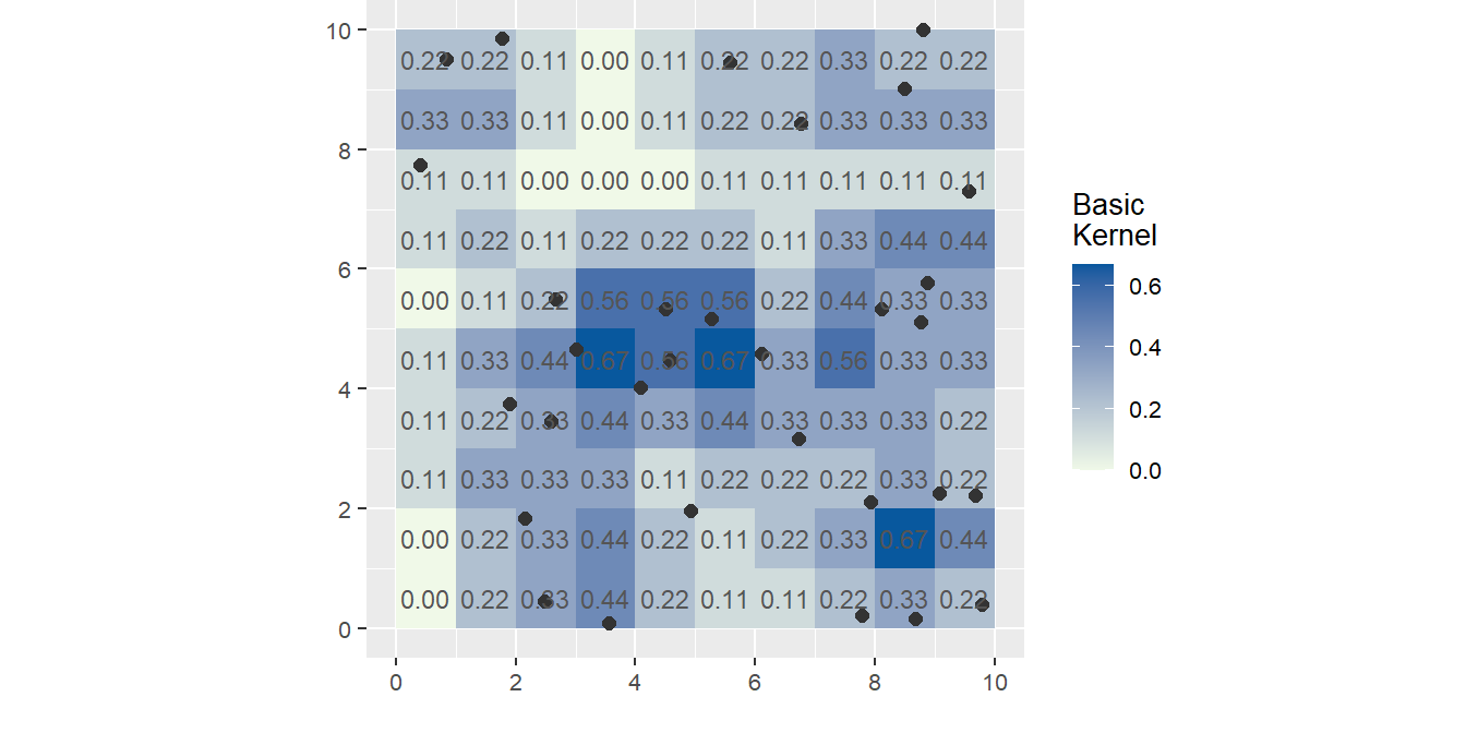
Kernel Density Function
TEs una técnica no paramétrica que permite estimar la intensidad local de un patrón de puntos en el espacio. En vez de contar cuántos puntos hay en un cuadrado (como en el método de cuadrantes), KDE suaviza la información de los puntos en un mapa continuo.

Kernel Density Function
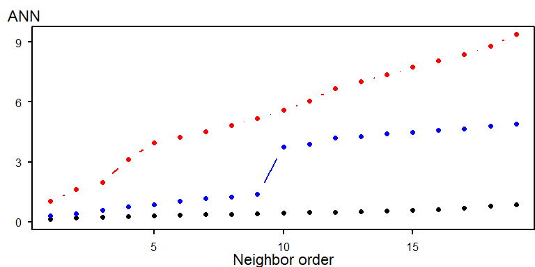
Análisis de vecino más cercano (NN)
El método compara la distribución espacial observada con una distribución teórica aleatoria. La herramienta de Vecino Más Cercano Promedio (ANN) mide la distancia entre el centroide de cada entidad y el centroide de su vecino más cercano. Luego promedia todas estas distancias al vecino más cercano. Si la distancia promedio es menor que la distancia promedio de una distribución aleatoria hipotética, se considera que la distribución de las entidades analizadas está agrupada. Si la distancia promedio es mayor que la de una distribución aleatoria hipotética, se considera que las entidades están dispersas.
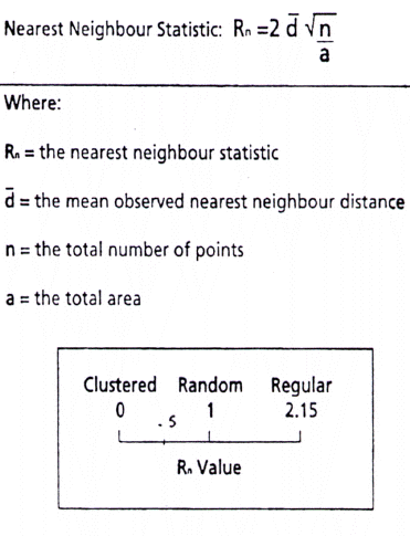
NN analysis

Análisis de vecino más cercano (NN)
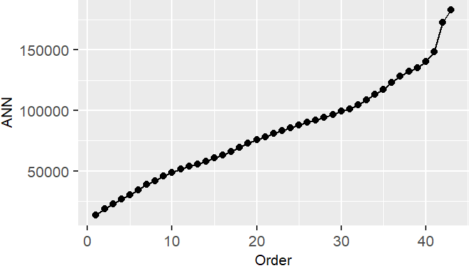
Una extensión de esta idea es graficar los valores de ANN para vecinos de diferente orden, es decir, para el punto más cercano, luego el segundo más cercano, y así sucesivamente.
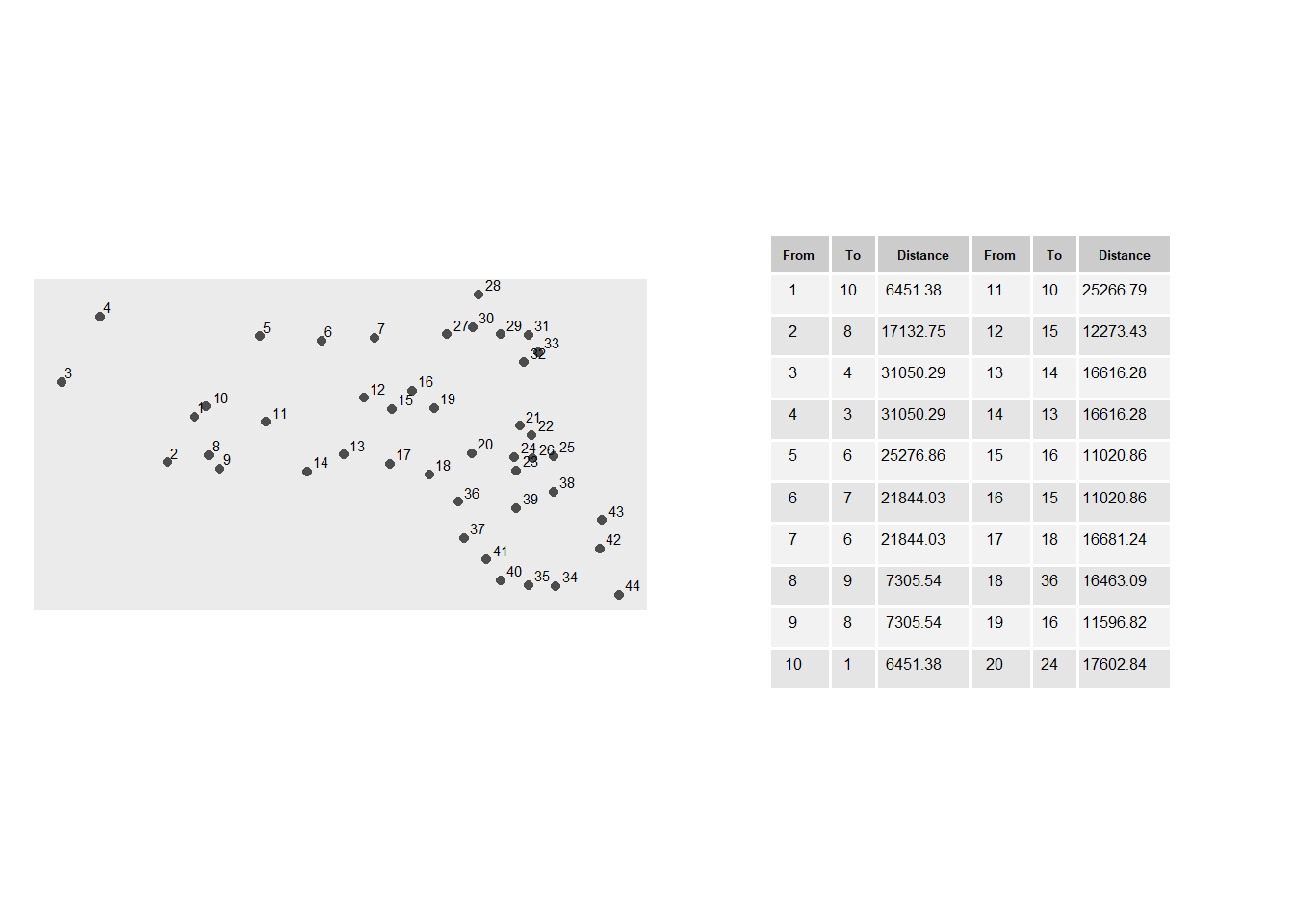
Análisis de vecino más cercano (NN)
Función K de Ripley
Es un método de análisis espacial para estudiar patrones de puntos basado en una función de distancia. El resultado de la función es el número esperado de eventos dentro de un radio \( d \). Se calcula como una serie de distancias incrementales \( d \) centradas, sucesivamente, en cada uno de los eventos.

Clustering
El objetivo es identificar subgrupos en los datos, de tal forma que los datos en cada subgrupo (clusters) sean muy similares, mientras que los datos en diferentes subgrupos sean muy diferentes.
Distance


- Hierarchical Clustering: descomposición jerárquica utilizando algún criterio, pueden ser aglomerativos (bottom-up) o de separación (top-down). No necesitan K al inicio.
- Partitioning Methods ( (k-means, PAM, CLARA): se construye a partir de particiones, las cuales son evaluadas por algún criterio. Necesitan K al inicio.
- Density-Based Clustering: basados en funciones de conectividad y funciones de densidad.
- Model-based Clustering: se utiliza un modelo para agrupar los modelos.
- Fuzzy Clustering: A partir de lógica difusa se separan o agrupan los clusters.

Clustering

Dendrograma

Dendrograma

Dendrograma


K-means


Método Silhouette

DBScan
DBSCAN is a density-based clustering method, which means that points that are closely packed together are assigned into the same cluster and given the same ID. The DBSCAN algorithm has two parameters, which the user needs to specify:
In short, all groups of at least minPts points, where each point is within ε or less from at least one other point in the group, are considered to be separate clusters and assigned with unique IDs. All other points are considered “noise” and are not assigned with an ID.
DBScan

Modelos Lineales Generalizados (GML)
Modelos Lineales Generalizados (GML)
Los Modelos Lineales Generalizados (GLM) son una extensión de los modelos lineales clásicos (como la regresión lineal) que permiten modelar una variedad más amplia de tipos de datos, incluyendo aquellos que no siguen una distribución normal. Estos modelos son especialmente útiles cuando la variable dependiente sigue una distribución distinta, como una distribución binomial (en el caso de variables de respuesta dicotómicas), una distribución de Poisson (para conteos), o una distribución gamma (para variables continuas positivas).
- Función de enlace (𝑔(⋅)): Establece la relación entre la media de la variable dependiente 𝑌 y los predictores lineales.
- Distribución de la variable dependiente: La variable dependiente 𝑌 sigue una distribución dentro de la familia exponencial (por ejemplo, normal, binomial, Poisson, etc.).
- Predictores lineales: La relación entre los predictores 𝑋1, 𝑋2,…,Xp y la variable dependiente se describe mediante una combinación lineal de los mismos.
\[g(\mathbb{E}[Y_i]) = \beta_0 + \beta_1 X_{i1} + \beta_2 X_{i2} + \dots + \beta_p X_{ip}\]
Modelos GLM
Regresión Lineal Gaussiana
\[ \mathbb{E}[Y_i] = \mu_i = \beta_0 + \beta_1 X_1 + \dots + \beta_p X_p \]
Regresión Logística
\[ \log\left(\frac{\mu_i}{1-\mu_i}\right) = \beta_0 + \beta_1 X_1 + \dots + \beta_p X_p \]
Regresión Poisson
\[ \log(\mu_i) = \beta_0 + \beta_1 X_1 + \dots + \beta_p X_p \]
Regresión Binomial Negativa
\[ \log(\mu_i) = \beta_0 + \beta_1 X_1 + \dots + \beta_p X_p \]
Regresión Logística
Distribución de la variable dependiente: Binomial \( Y_i \sim \text{Binomial}(n, \mu_i) \)
Función de enlace: Logit (función logística)
Formulación matemática:
\[ \log\left(\frac{\mu_i}{1-\mu_i}\right) = \beta_0 + \beta_1 X_1 + \beta_2 X_2 + \dots + \beta_p X_p \]
Este modelo se utiliza cuando la variable dependiente es binaria (por ejemplo, éxito o fracaso).


Odds

Limitaciones de los Odds

Función LOGIT
Sea p(x) la probabilidad de éxito cuando el valor de la variable predictora es x, entonces:
Donde $a$ es el intercepto del modelo, $b$ son los coeficientes del modelo de regresión logística, y $x$ son las variables independientes (predictoras).
$P(y=1) = \frac{1}{1+e^{-(a+\sum bx)}}$Donde, P es la probabilidad de Bernoulli que una unidad de terreno pertenece al grupo de no deslizamientos o al grupo de si deslizamiento. P varía de 0 a 1 en forma de curva “S” (logística).
Odds

Regresión Logística

Regresión Logística

Regresión Logística

Resultado

$R^2$

$R^2$

$R^2$

Regresión con Poisson
Distribución de la variable dependiente: Poisson \( Y_i \sim \text{Poisson}(\mu_i) \)
Función de enlace: Logaritmo natural
Formulación matemática:
\[ \log(\mu_i) = \beta_0 + \beta_1 X_1 + \beta_2 X_2 + \dots + \beta_p X_p \]
Este modelo se utiliza cuando la variable dependiente representa un conteo de eventos en un intervalo de tiempo o espacio.
GLM de Poisson
A Poisson distribution is a discrete probability distribution, meaning that it gives the probability of a discrete (i.e., countable) outcome. For Poisson distributions, the discrete outcome is the number of times an event occurs, represented by $k$. You can use a Poisson distribution if:
- Individual events happen at random and independently. That is, the probability of one event doesn’t affect the probability of another event.
- You know the mean number of events occurring within a given interval of time (1D) or space (2D). This number is called $λ$ (lambda), and it is assumed to be constant.
- Two events cannot occur at exactly the same instant or place.
Distribución de Poisson
$$ P(Y_i = y_i) = \frac{\lambda_i^{y_i} e^{-\lambda_i}}{y_i!}, \quad y_i = 0, 1, 2, \ldots $$El modelo lineal generalizado (GML) de Poisson se especifica de la siguiente manera:
$$ \lambda_i = \mathbb{E}[Y_i] = e^{\eta_i}, \eta_i = \beta_0 + \beta_1 x_{i1} + \beta_2 x_{i2} + \cdots + \beta_p x_{ip} $$La función de enlace que relaciona la media $\lambda_i$ con la parte lineal $\eta_i$ es:
$$ \eta_i = \log(\lambda_i) $$De esta forma, la media de la distribución de Poisson se relaciona exponencialmente con la combinación lineal de las covariables:
$$ \lambda_i = e^{\beta_0 + \beta_1 x_{i1} + \beta_2 x_{i2} + \cdots + \beta_p x_{ip}} $$Poisson

Poisson

Regresión Binomial Negativa
Distribución de la variable dependiente: Binomial Negativa \( Y_i \sim \text{NegBin}(\mu_i, \theta) \)
Función de enlace: Logaritmo natural
Formulación matemática:
\[ \log(\mu_i) = \beta_0 + \beta_1 X_1 + \beta_2 X_2 + \dots + \beta_p X_p \]
Este modelo se utiliza cuando la variable dependiente es un conteo de eventos, pero hay sobredispersión (la varianza es mayor que la media), lo que no se captura adecuadamente con el modelo de Poisson.
Tipos de ceros en datos de conteo
Cuando modelamos eventos como deslizamientos, los ceros en los datos pueden surgir de al menos tres fuentes:
Ceros estructurales (verdaderos ceros)
Ejemplo: Lugares donde realmente no pueden ocurrir deslizamientos (e.g., lagos, llanuras totalmente estables).
Ceros aleatorios (cero por casualidad)
Ejemplo: Zonas propensas a deslizamientos donde podrían haber ocurrido, pero no ocurrieron durante el periodo observado.
Ceros por omisión o errores de observación
Ejemplo: Eventos que sí ocurrieron, pero no se registraron por limitaciones en los inventarios (e.g., imágenes satelitales de baja resolución) o falta de monitoreo.
Modelos Zero-Inflated
Los modelos de conteo clásicos como Poisson o binomial negativa suponen que los ceros ocurren como parte del proceso natural. Pero en muchos contextos reales (como deslizamientos), hay más ceros de los que esos modelos predicen.
- Una parte binaria (modelo logístico) que predice la probabilidad de estar en el grupo "siempre cero".
- Una parte de conteo (binomial negativa) que modela el número de eventos si no está en el grupo "siempre cero".
Areal data
Discrete
Geovisualización
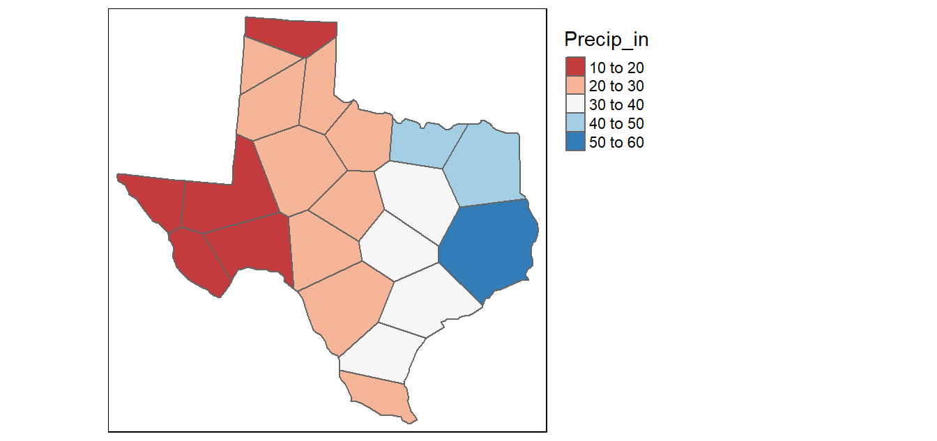
Choropleth maps
Choropleth maps are thematic maps in which areas are rendered according to the values of the variable displayed
Cloropleth maps are used to obtain a graphical perspective of the spatial distribution of the values of a specific variable across the study area.
There are two main categories of variables displayed in choropleth maps:
- Spatially extensive variables: each polygon is rendered based on a measured value that holds for the entire polygon. Ej. total population
- Spatially intensive variables: the values of the variable are adjusted for the area or some other variable. Ej. population density
Choropleth maps
Breaks
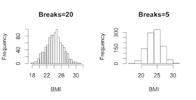
Breaks

Breaks

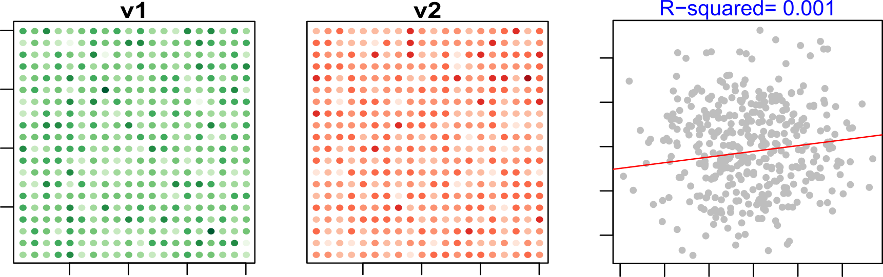
Spatial association
Spatial dependence
Formal property that measures the degree to which near and distant things are related
Refers to systematic spatial changes that are observed as clusters of similar values or a systematic spatial pattern.
Spatial heterogeneity
Spatial heterogeneity refers to structural relationships that change with the location of the object. These changes can be abrupt (e.g. countryside–town) or continuous.
Spatial heterogeneity refers to the uneven distribution of a trait, event, or relationship across a region
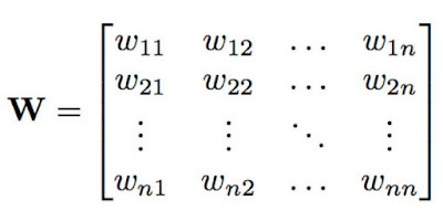
Spatial weight matrix (W)
Spatial weights are numbers that reflect some sort of distance, time or cost between a target spatial object and every other object in the dataset or specified neighborhood. Spatial weights quantify the spatial or spatiotemporal relationships among the spatial features of a neighborhood.
Neighborhood
Neighborhood in the spatial analysis context is a geographically localized area to which local spatial analysis and statistics are applied based on the hypothesis that objects within the neighborhood are likely to interact more than those outside it.
- Neighbours by contiguity: areas that share common boundaries
- neighbours by distance: areas will be defined as neighbours if they are within a specified radius
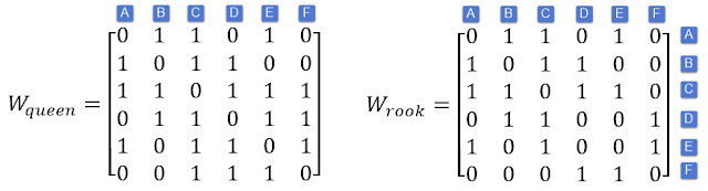
Spatial Relationships
Adjacency (Contiguity)
Adjacency can be thought of as the nominal, or binary, equivalent of distance. Two spatial entities are either adjacent or they are not.
Contiguity among features means the features have common borders. We have three types of contiguity:
- Rook Contiguity: the features share common edges
- Bishop Contiguity: the features share common vertices (corners)
- Queen Contiguity: the feature share common edges and corners.
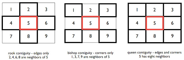
Contiguity


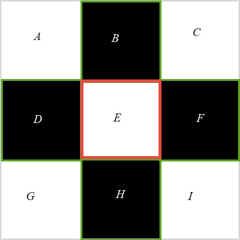
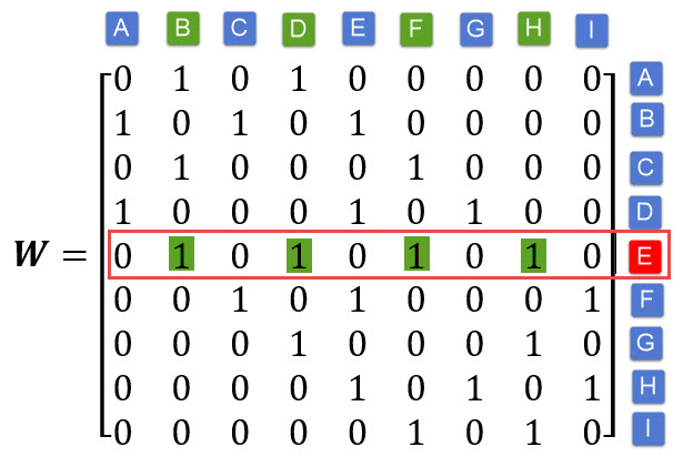
Ej.

Matrix of k nearest neighbours (knn)

Standarized Spatial Weights
Row standardization is recommended when there is a potential bias in the distribution of spatial objects and their attribute values due to poorly designed sampling procedures.
Row standardization should also be used when polygon features refer to administrative boundaries or any type of man-made zones.
Ej.

Spatial lag
Spatial lagis when the dependent variable y in place i is affected by the independent variables in both place i and j.


Global indicator of Spatial Association (GISA)
The measures (test statistics) related to the existence of spatial autocorrelation in data, that is, focusing on whether there is any spatial autocorrelation in the data
Indice de Moran
The positive value of global Moran implies the existence of a positive autocorrelation, and conversely, the negative value implies the existence of a negative autocorrelation

If there is no relationship between Income and Income_lag, the slope will be close to flat (resulting in a Moran’s I value near 0).


Moran’s I at different lags
Moran’s I at different spatial lags defined by a 50 km width annulus at 50 km distance increments. Red dots indicate Moran I values for which a P-value was 0.05 or less.
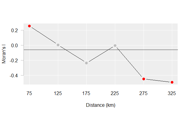
Moran’s I at different lags

Moran’s I at different lags

Moran’s I at different lags

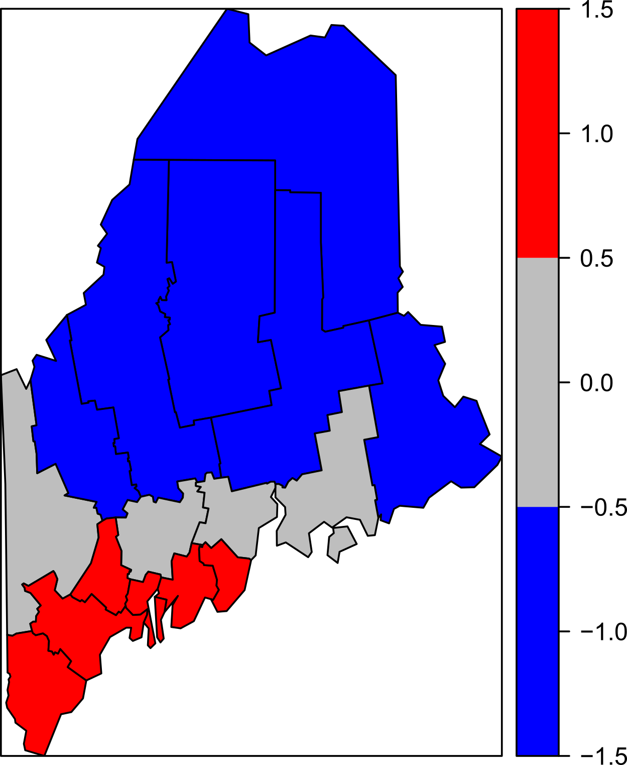
Local indicators of Spatial Association (LISA)
A local statistic is any descriptive statistic associated with a spatial data set whose value varies from place to place.

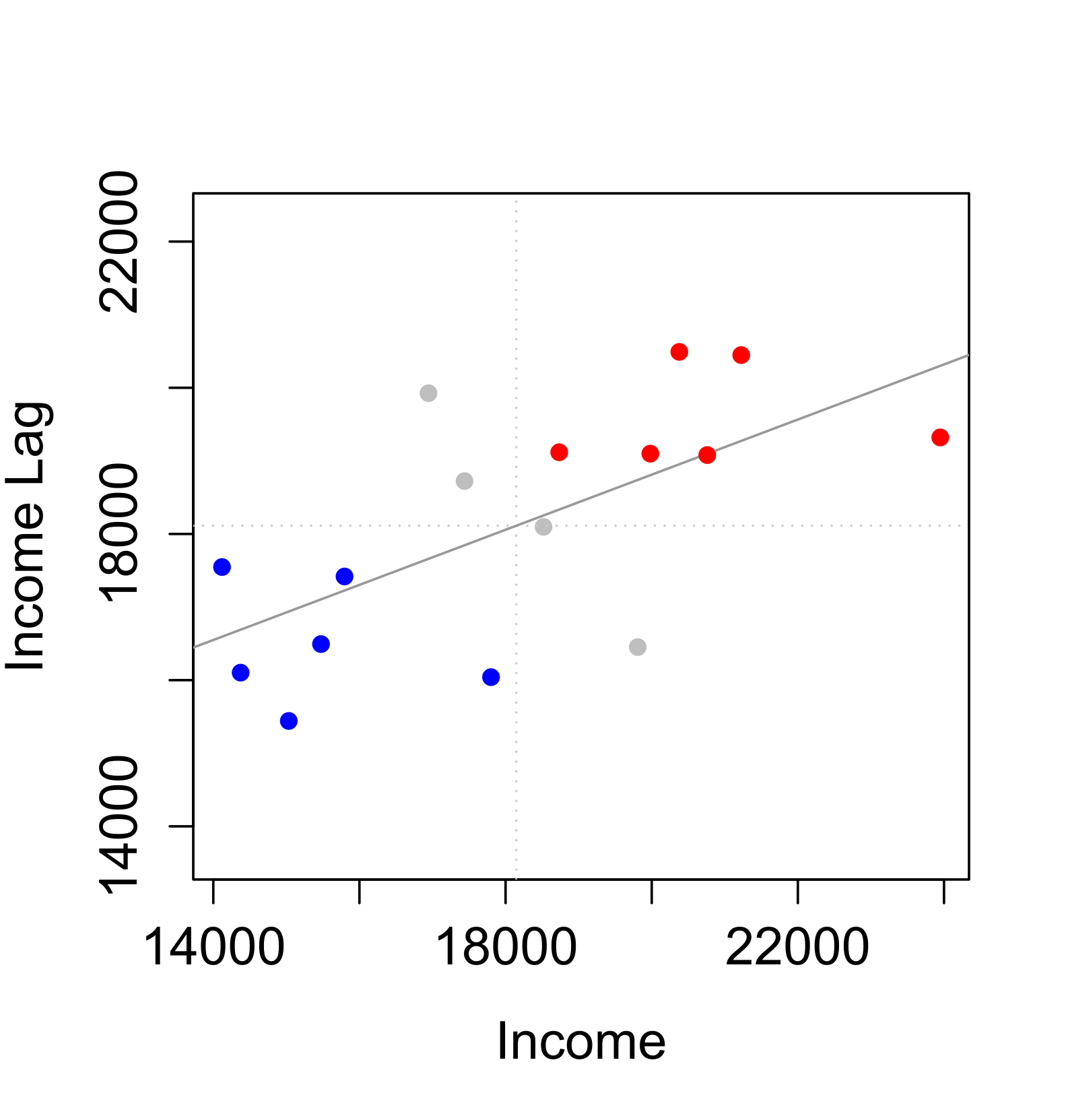
Moran´s I scatter plot

Moran´s I scatter plot
Red points and polygons highlight counties with high income values surrounded by high income counties. Blue points and polygons highlight counties with low income values surrounded by low income counties.
Moran´s I scatter plot

Moran´s I scatter plot

Moran´s I scatter plot

Spatial cluster

Spatial Regression Models
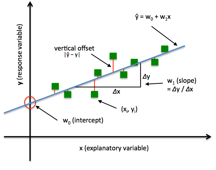
Simple Linear Regression model
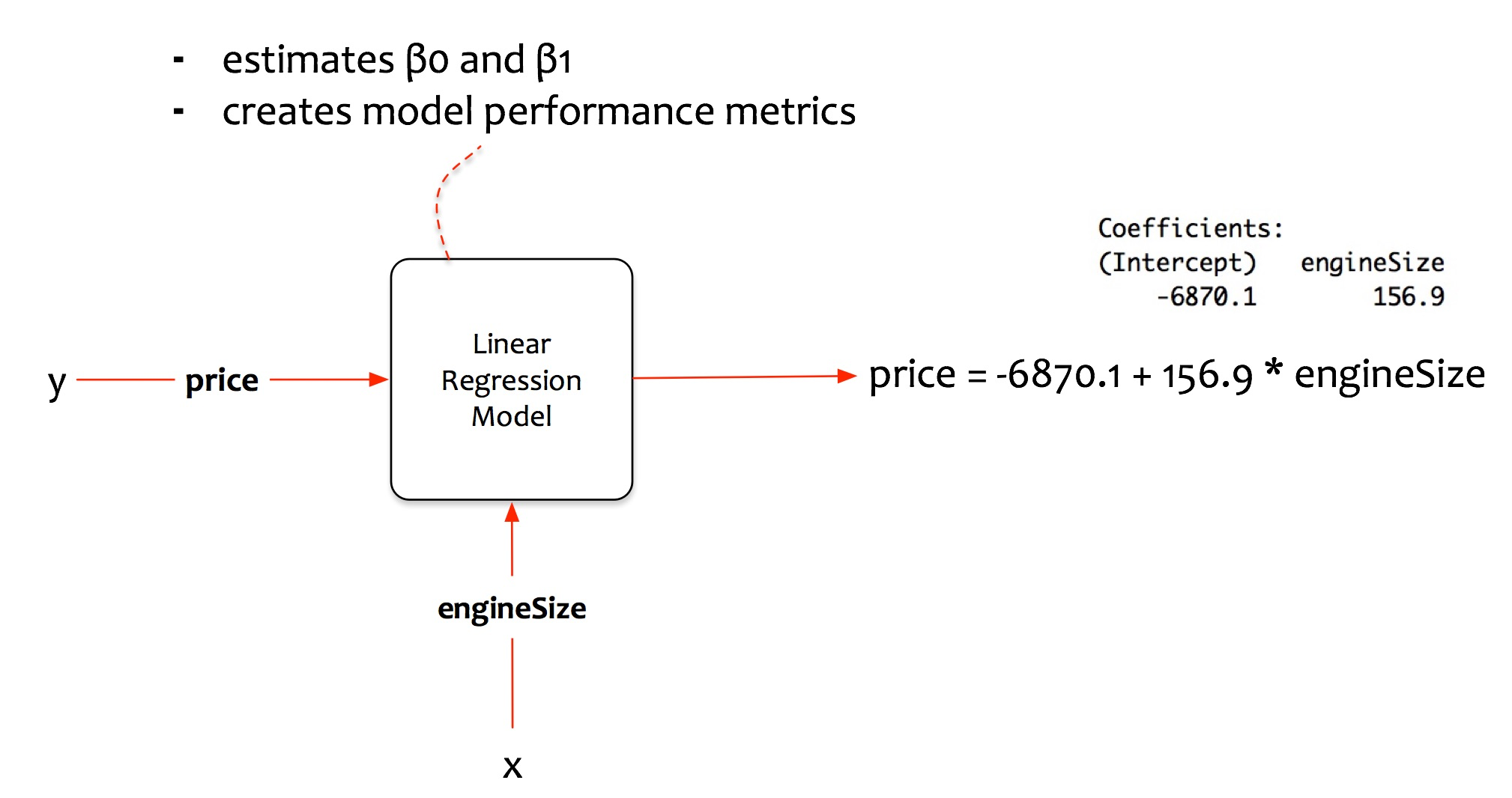
Regresión lineal
Multivariate regression model
Multivariate regression model
Ordinary least squares regression (OLS)
Assumptions
- Linear relationship between the dependent and independent variables
- Multivariate normality: the residual of the linear model should be normally distributed
- No multicolinearity between independent variables, i.e. they should not correlate between each other
- Homoscedasticity: the errors/residuals should have constant variance (no trends)
- No autocorrelation: residuals (errors) in the model shoul not be correlqated in any way
Resultados
$R^2$

Adjusted $R^2$
Spatial regression

Spatial regression

Modelos de regresión para Heterogeneidad Espacial
Regimenes Espaciales
Simson`s paradox

Simson`s paradox

Simson`s paradox

Heterogeneidad espacial

Heterogeneidad espacial

Heterogeneidad espacial

Modelos multiniveles (jerárquicos)

No jerarquico

Random intercepto (fixed effect)

Random slope (regimes)

Random slope & intercepto

Modelo multinivel - fixed effect

Modelo multinivel - regimenes

Modelo multinivel

Intraclass Correlation Coefficient
\[ Y_{ij} = \beta_0 + \beta_1 X_1 + \mu_j + \epsilon_{ij} \]
\[\mu_j = iid, N(0,\sigma_0^2)\]
\[\epsilon_{ij} = iid, N(0,\sigma^2)\]
where $Y_{ij}$ is the dependent variable for individual $i$ in group $j$, $X_1$ is an independent variable, $β_0$ is the overall intercept, $β_1$ is the coefficient for the independent variable, $μ_j$ is the random effect for group $j$, and $ε_{ij}$ is the residual error term for individual $i$ in group $j$.
\[ Cov(Y_{ij},Y_{ji}) = \mu_j\ = \sigma_0^2 \]
\[ Corr(Y_{ij},Y_{ji}) = \frac{\sigma_0^2}{\sigma_0^2+\sigma^2} \]
Intraclass Correlation Coefficient
La Correlación Intraclase es la razón entre la varianza entre grupos y la varianza total. Te indica la proporción de la varianza total en Y que es explicada por la agrupación en conglomerados. También puedes interpretarla como la correlación entre las observaciones dentro del mismo grupo.
\[ Corr(Y_{ij},Y_{ji}) = \frac{\sigma_0^2}{\sigma_0^2+\sigma^2} \]
Geographycally Weighted Regresion (GWR)
Geographycally Weighted Regresion (GWR)
where $(ui, vi)$ are the spatial coordinates of the observations $i$, and $β_k (ui, vi)$ are the coefficients estimated at those locations.
Thus, in contrast to global LRMs, GWR conducts local regression at a series of locations to estimate local coefficients (the geographical part of GWR), using observations weighted by their distances to the location at the center of the moving window/kernel (the weighted part).
Parameters
Bandwidth is the distance band or number of neighbors used for each local regression equation and is perhaps the most important parameter to consider for Geographically Weighted Regression, as it controls the degree of smoothing in the model.
It can be based on either Number of Neighbors or Distance Band. When Number of Neighbors is used, the neighborhood size is a function of a specified number of neighbors, which allows neighborhoods to be smaller where features are dense and larger where features are sparse. When Distance Band is used, the neighborhood size remains constant for each feature in the study area, resulting in more features per neighborhood where features are dense and fewer per neighborhood where they are sparse.
Parameters
The power of GWR is that it applies a geographical weighting to the features used in each of the local regression equations. Features that are farther away from the regression point are given less weight and thus have less influence on the regression results for the target feature; features that are closer have more weight in the regression equation. The weights are determined using a kernel, which is a distance decay function that determines how quickly weights decrease as distances increase. The Geographically Weighted Regression tool provides two kernel options in the Local Weighting Scheme parameter, Gaussian and Bisquare.
Single bandwidth
a single bandwidth is used in GWR under the assumption that the response-to-predictor relationships operate over the same scales for all of the variables contained in the model. This may be unrealistic because some relationships can operate at larger scales and others at smaller ones. A standard GWR will nullify these differences and find a “best-on-average” scale of relationship non-stationarity (geographical variation)
Geographycally Weighted Regresion (GWR)

Geographycally Weighted Regresion (GWR)
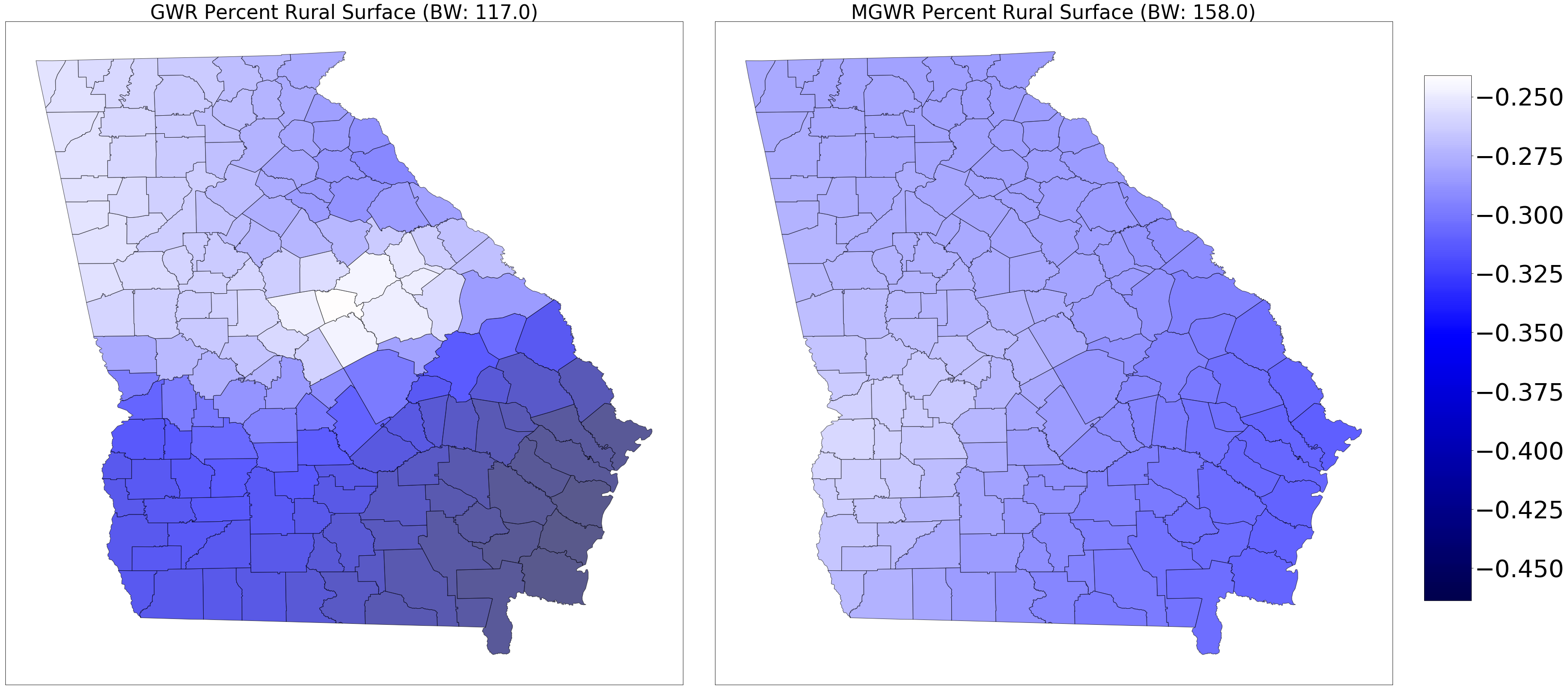
Adaptativo

Fijo (distancia)

Distribución del error
Modelos de regresión para Dependencia Espacial
Modelos autoregresivos SAR
SAR
SAR models account for spatial dependence by including a spatial lag of the dependent variable, error term or exogenous variables. Essentially, they add an autoregressive component that takes into account the weighted average of neighboring values. SAR models are typically specified in the form:
$y = \rho Wy + X\beta + \epsilon$
Joint Distribution in SAR
The SAR model’s joint distribution of the spatial effects y is derived directly from this equation:
$y=(I−ρW)^{−1}(Xβ+ϵ)$
SAR uses a single, global equation involving W to directly specify the joint distribution across all locations.
Dense covariance matrix ($\sum$)
$\sum=(I-\rho W)^{-1}(I-\rho W)^{-T}$


SAR
SAR is formulated as a global process, where the spatial relationships affect the entire dataset simultaneously. The SAR model requires matrix inversion, which can be computationally challenging for large datasets.
SAR Models interpret the spatial effects by including a lag term of the dependent variable, capturing how the value at one location is influenced by the values of all its neighbors. This kind of specification is more aligned with the concept of spatial spillover, meaning that the outcome in one region directly influences the outcomes in neighboring regions.
Modelos autoregresivos

Modelos autoregresivos

Modelos autoregresivos CAR
CAR
CAR models are based on a conditional specification of the dependent variable. Unlike SAR, the CAR model is defined using the conditional distribution of a particular value, given the values of its neighbors. CAR models are generally written in the form:
$y_i=X_iβ+y_i∣y_{-i}+ϵ_i$
$y_i∣y_{-i} ∼N(∑_jϕ_{ij}y_j,τ^2)$
CAR
CAR is formulated using local conditional distributions. This approach leads to a specification where the model conditions on neighboring units, making CAR easier to interpret in a local spatial context. The precision matrix (inverse of the covariance matrix) in a CAR model has a sparse structure, which often makes CAR models more computationally efficient, especially for large spatial datasets.
Precision matrix
$Q=D-W$
Donde D es el número de vecinos

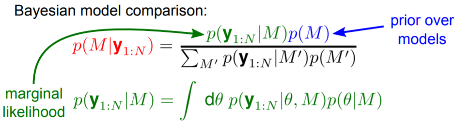
Bayes's theorem

Teorema de Bayes
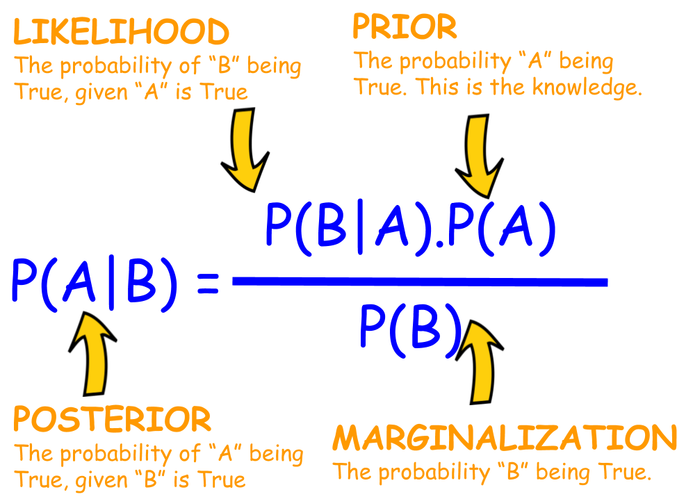


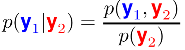
Conditional probability
A conditional probability is a probability that measures the probability of one event given another event. Intuitively, it is just a proportion of event A’s probability under the occurrence of event B’s.

Joint probability
A joint probability is a probability that calculates probabilities (or likelihoods) of two events that co-occur.

Marginal probability
A marginal probability is a probability of a single event occurring. When a single event occurs with other events, we can decompose it by joint probability with each event.

Joint Distribution in CAR
In the CAR model, although we don’t specify the joint distribution directly, we can derive it from the set of conditional distributions using properties of Markov Random Fields.
The resulting joint distribution for $u$ in a CAR model is represented by a precision matrix (inverse of the covariance matrix), which is sparse. This sparse structure means that only neighboring locations have direct dependencies, unlike SAR’s dense structure.
Mathematically, the joint distribution of $u$ in a CAR model can be expressed as:
$P(u) \propto \exp \left( -\frac{1}{2} u^T Q u \right)$
Intrinsic CAR models (ICAR)
In ICAR models, the precision matrix Q is often singular (non-invertible), which means that the joint distribution does not have a unique covariance matrix. This results in non-identifiability of the random effects in an absolute sense.
To make the model identifiable, ICAR models typically impose a constraint on the spatial random effects, such as a sum-to-zero constraint (e.g., $\sum u_i = 0$). This allows for relative spatial effects, where the values are interpreted relative to the mean of the spatial region rather than as absolute values.
Locally Dependent Structure: In ICAR, the random effect at each location depends only on the neighboring locations, not on any fixed “global” effect. This is why ICAR models are often preferred for applications that require purely local dependencies.
Leroux CAR
Flexible Precision Matrix: The Leroux CAR model has a precision matrix that can be adjusted to avoid singularity, making it possible to estimate a proper covariance structure.
Mixing Parameter: A parameter $\lambda$ (often called the spatial dependence parameter) controls the strength of spatial dependence: (i) If $\lambda = 1$, the model behaves like an ICAR model, with strong spatial dependence. (ii) If $\lambda = 0$, the model assumes independence across locations. (iii) For values between 0 and 1, the model interpolates between independence and spatial dependence, allowing for partial spatial smoothing.
Proper Priors: By adjusting $\lambda$, the Leroux CAR can provide a proper (non-singular) prior distribution, which can help in avoiding identifiability issues and allows the covariance structure to be better specified.
Besag-York-Mollié (BYM) Model
This model combines ICAR for spatial effects and unstructured random effects, allowing for both spatially structured and unstructured variability.
Interpretación de la dependencia espacial
La dependencia espacial puede interpretarse de dos formas:
- Omitir variables (latent): dependencia debida a factores no observados.
- Interacción con vecinos (spillover): resultado del proceso de interacción espacial.
| Modelo | Tipo de dependencia | ¿Spillover observable? | ¿Estructura latente? |
|---|---|---|---|
| SAR (Spatial Autoregressive) |
Global (interacción en WY) | Sí | No |
| SDM (Spatial Durbin Model) |
Global + local (WY y WX) | Sí | No |
| CAR (Conditional Autoregressive) |
Local condicional (Yi | Yj) | No | Sí |
Interpretación clave del modelo CAR
- No implica causalidad ni retroalimentación espacial.
- Captura autocorrelación en los efectos aleatorios espaciales.
Field model
Continuos
Geostatistics
Geostatistics
The type of spatial statistical analysis dealing with continuous field variables is named “geostatistics”
Geostatistics focus on the description of the spatial variation in a set of observed values and on their prediction at unsampled locations
Spatial interpolation
techniques used with points that represent samples of a continuous field are interpolation methods
Here, our point data represents sampled observations of an entity that can be measured anywhere within our study area
There are many interpolation tools available, but these tools can usually be grouped into two categories: deterministic and interpolation methods
Proximity interpolation
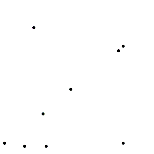
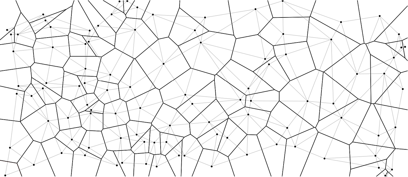
It was introduced by Alfred H. Thiessen more than a century ago. The goal is simple: Assign to all unsampled locations the value of the closest sampled location. This generates a tessellated surface whereby lines that split the midpoint between each sampled location are connected thus enclosing an area. Each area ends up enclosing a sample point whose value it inherits.
Voronoi diagram
Voronoi & Delanauy triangulation
Inverse Distance Weighted (IDW)
The IDW technique computes an average value for unsampled locations using values from nearby weighted locations. The weights are proportional to the proximity of the sampled points to the unsampled location and can be specified by the IDW power coefficient.
$\hat{Z_j} = \frac{\sum_i{Z_i / d ^ n_{ij}}}{\sum_i{1 / d ^ n_{ij}}}$So a large n results in nearby points wielding a much greater influence on the unsampled location than a point further away resulting in an interpolated output looking like a Thiessen interpolation. On the other hand, a very small value of n will give all points within the search radius equal weight such that all unsampled locations will represent nothing more than the mean values of all sampled points within the search radius.
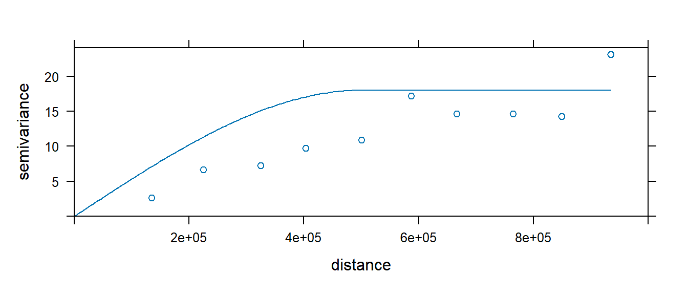
Kriging
Several forms of kriging interpolators exist: ordinary, universal and simple just to name a few. This section will focus on ordinary kriging (OK) interpolation. This form of kriging usually involves four steps:
- Removing any spatial trend in the data
- Computing the experimental variogram, $γ$ , which is a measure of spatial autocorrelation.
- Defining an experimental variogram model that best characterizes the spatial autocorrelation in the data.
- Interpolating the surface using the experimental variogram.
- Adding the kriged interpolated surface to the trend interpolated surface to produce the final output.
We are interested in how these attribute values vary as the distance between location point pairs increases. We can compute the difference, $γ$, in values by squaring their differences then dividing by 2.
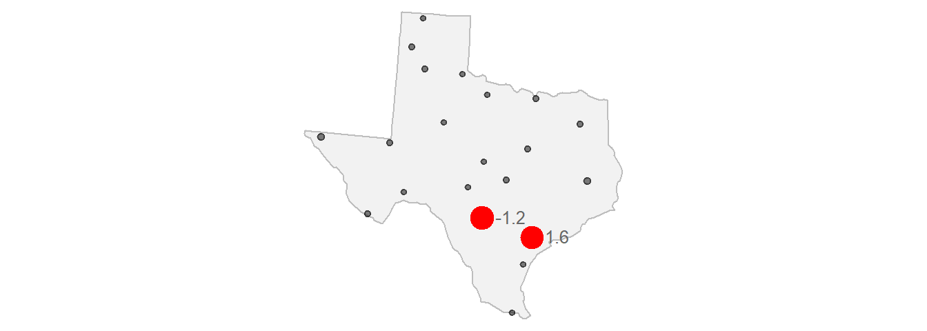 $\gamma = \frac{(Z_2 - Z_1) ^ 2}{2} = \frac{(-1.2 - (1.6)) ^ 2}{2} = 3.92$
Experimental variogram
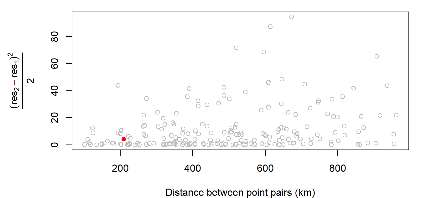
Experimental variogram
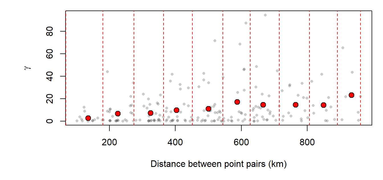
Experimental semivariogram
Variogram models
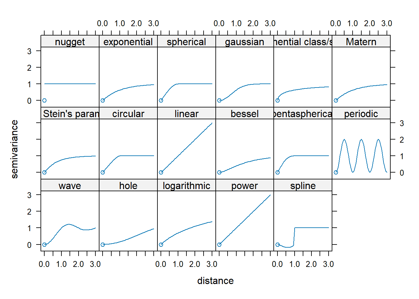
Variogram models
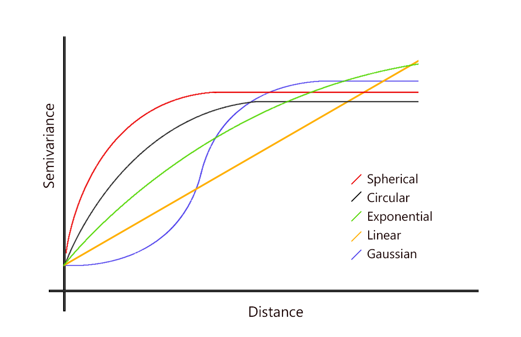
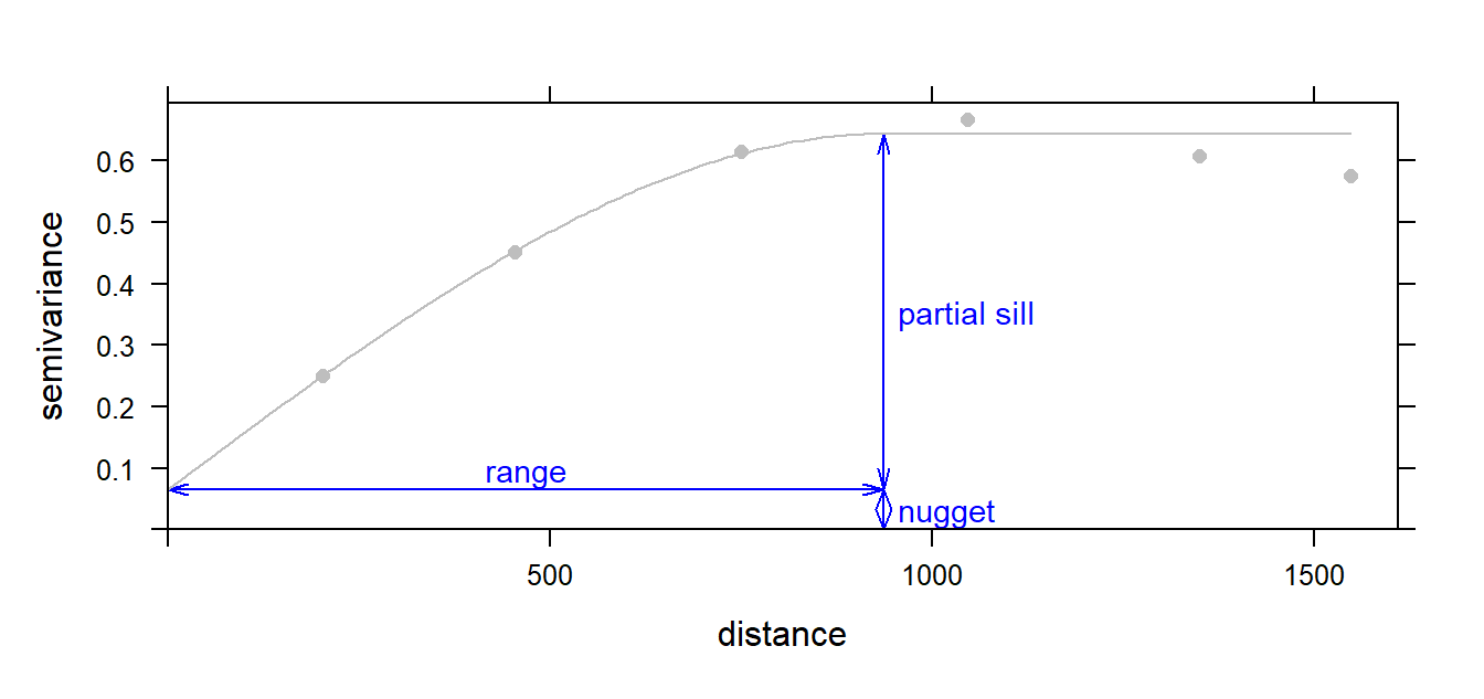
Parameters in a variogram model
Spherical model fit
Gaussian Processes
Spatial Gaussian process (SGP)
A spatial Gaussian process (SGP) refers to a stochastic process frequently employed to model data exhibiting spatial, temporal, or spatiotemporal dependence. A common approach to modeling process $Y(s)$ is by utilizing a spatial linear mixed effects model:
$Y(s)=\mu(s)+w(s)+\epsilon(s)$
the residual component can be decomposed into two parts: a spatial component ($w(s)$) and a unstructured component ($\epsilon(s)$) $iid$. The spatial component can be modeled as a stationary spatial Gaussian process with zero mean and a covariance function $w(s)~SGP(0,\sum)$.
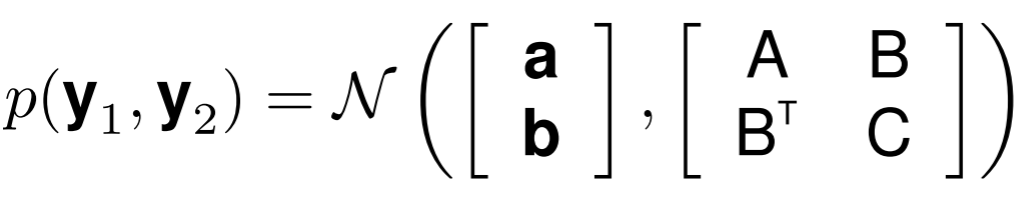
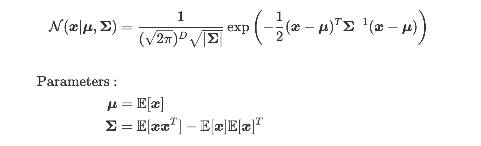
Distribución Gaussiana multivariada
Multivariate Gaussian distribution is the joint probability of Gaussian distribution with more than two dimensions. It has the probability density function below.

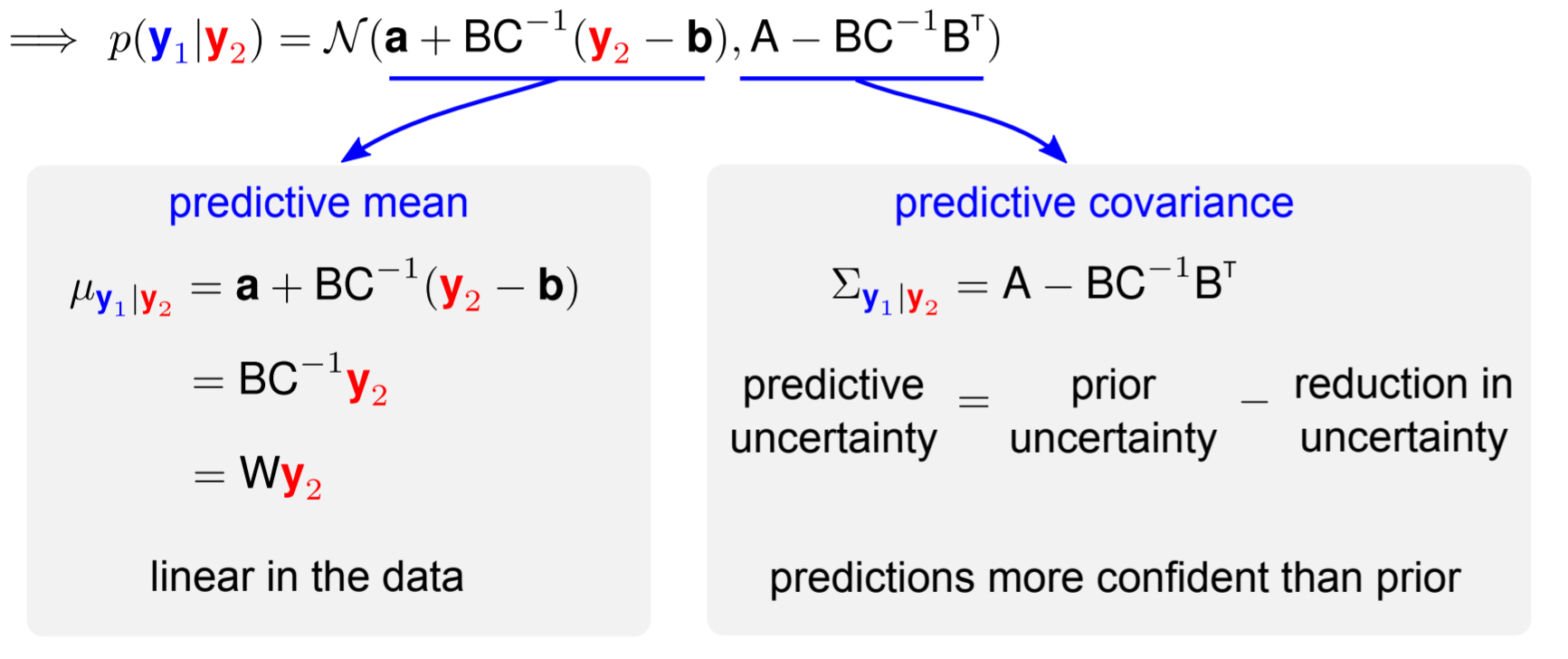
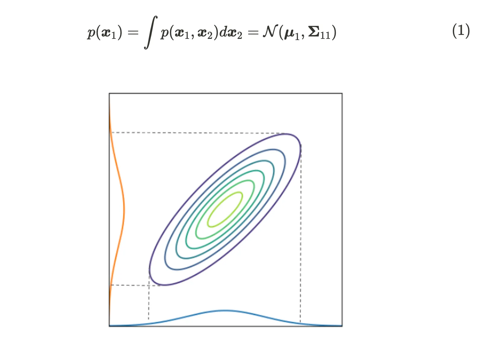
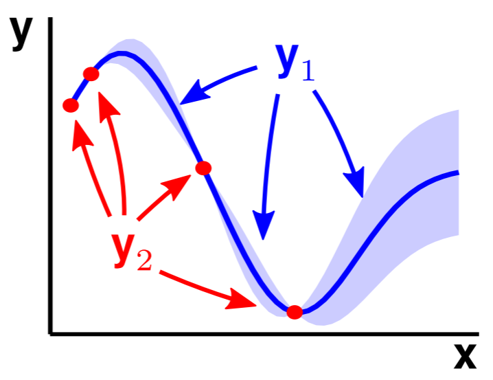
Distribución marginal

Distribución condicionada

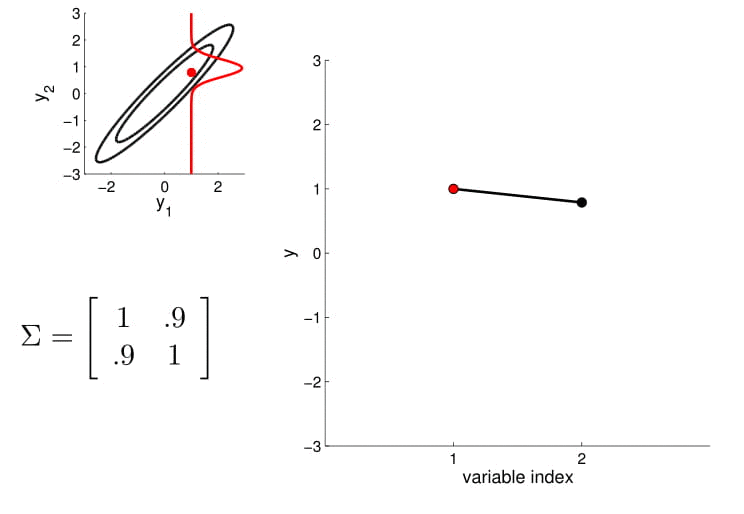
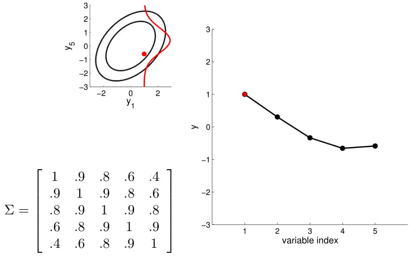
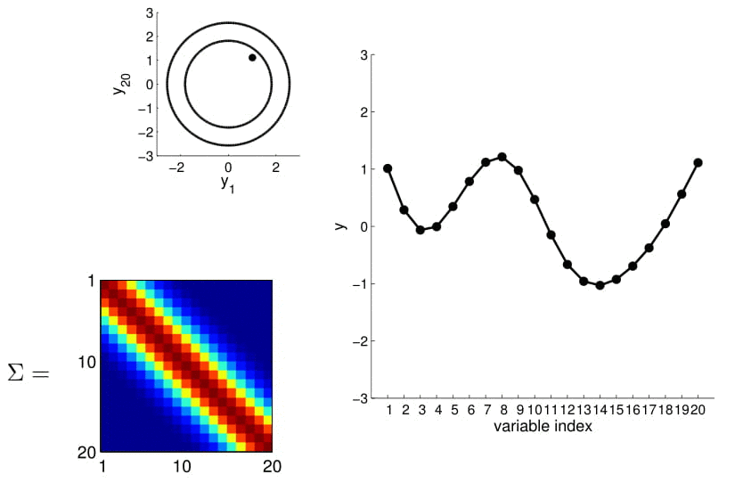
Matriz de covarianza
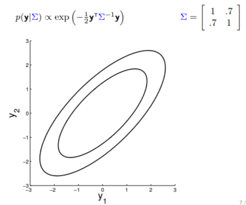
Matriz de covarianza
Matriz de covarianza
2D Gaussian
2D Gaussian
2D Gaussian
5D Gaussian
5D Gaussian
20D Gaussian
20D Gaussian
20D Gaussian
Gaussian Process (infinite D)
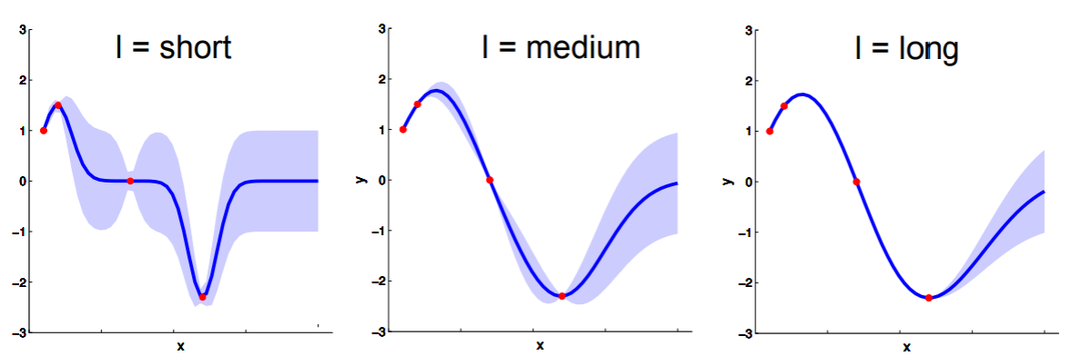
Hiper-parámetros
Hiper-parámetros
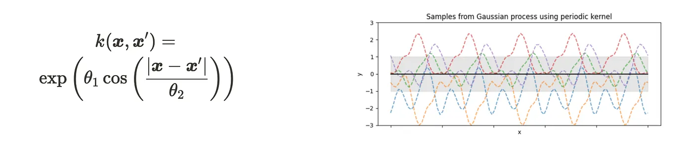
Kernel

Kernel
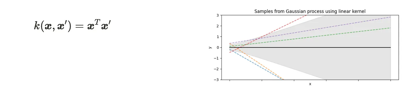
Kernel
Nuevos datos
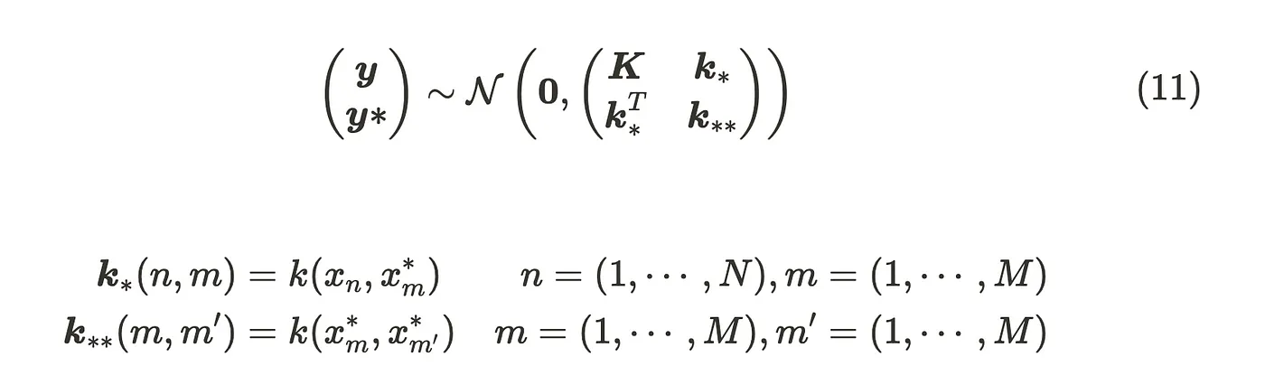

Predicción
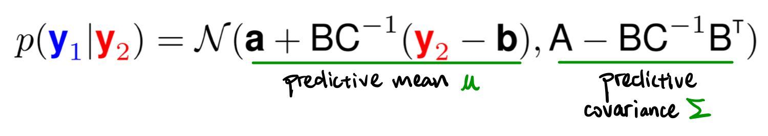
Predicción

Predicción